ML | Kaggle Breast Cancer Wisconsin Diagnosis using KNN and Cross Validation (original) (raw)

Last Updated : 22 May, 2024

**Dataset :**It is given by Kaggle from UCI Machine Learning Repository, in one of its challenges. It is a dataset of Breast Cancer patients with Malignant and Benign tumor. K-nearest neighbour algorithm is used to predict whether is patient is having cancer (Malignant tumour) or not (Benign tumour). Implementation of KNN algorithm for classification. Code : Importing Libraries

Python3 1== `

performing linear algebra

import numpy as np

data processing

import pandas as pd

visualisation

import matplotlib.pyplot as plt

Code : Loading dataset

Python3 1== `

df = pd.read_csv("..\breast-cancer-wisconsin-data\data.csv")

print (data.head)

Output : 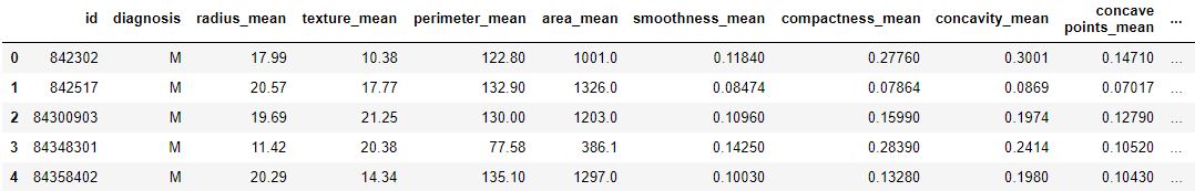Code: Data Info

Python3 1== `

df.info()

Output :

RangeIndex: 569 entries, 0 to 568 Data columns (total 33 columns): id 569 non-null int64 diagnosis 569 non-null object radius_mean 569 non-null float64 texture_mean 569 non-null float64 perimeter_mean 569 non-null float64 area_mean 569 non-null float64 smoothness_mean 569 non-null float64 compactness_mean 569 non-null float64 concavity_mean 569 non-null float64 concave points_mean 569 non-null float64 symmetry_mean 569 non-null float64 fractal_dimension_mean 569 non-null float64 radius_se 569 non-null float64 texture_se 569 non-null float64 perimeter_se 569 non-null float64 area_se 569 non-null float64 smoothness_se 569 non-null float64 compactness_se 569 non-null float64 concavity_se 569 non-null float64 concave points_se 569 non-null float64 symmetry_se 569 non-null float64 fractal_dimension_se 569 non-null float64 radius_worst 569 non-null float64 texture_worst 569 non-null float64 perimeter_worst 569 non-null float64 area_worst 569 non-null float64 smoothness_worst 569 non-null float64 compactness_worst 569 non-null float64 concavity_worst 569 non-null float64 concave points_worst 569 non-null float64 symmetry_worst 569 non-null float64 fractal_dimension_worst 569 non-null float64 Unnamed: 32 0 non-null float64 dtypes: float64(31), int64(1), object(1) memory usage: 146.8+ KB

Code: We are dropping columns - 'id' and 'Unnamed: 32' as they have no role in prediction

Python3 1== `

df.drop(['Unnamed: 32', 'id'], axis = 1) print(df.shape)

Output:

(569, 31)

Code: Converting the diagnosis value of M and B to a numerical value where M (Malignant) = 1 and B (Benign) = 0

Python3 1== `

def diagnosis_value(diagnosis): if diagnosis == 'M': return 1 else: return 0

df['diagnosis'] = df['diagnosis'].apply(diagnosis_value)

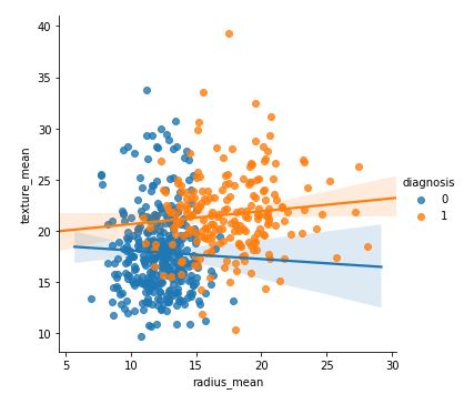
Code :

Python3 1== `

sns.lmplot(x = 'radius_mean', y = 'texture_mean', hue = 'diagnosis', data = df)

Output:

Code :

Python3 1== `

sns.lmplot(x ='smoothness_mean', y = 'compactness_mean', data = df, hue = 'diagnosis')

Output: 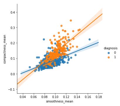Code : Input and Output data

Python3 1== `

X = np.array(df.iloc[:, 1:]) y = np.array(df['diagnosis'])

Code : Splitting data to training and testing

Python3 1== `

from sklearn.model_selection import train_test_split X_train, X_test, y_train, y_test = train_test_split( X, y, test_size = 0.33, random_state = 42)

Code : Using Sklearn

Python3 1== `

knn = KNeighborsClassifier(n_neighbors = 13) knn.fit(X_train, y_train)

Output:

KNeighborsClassifier(algorithm='auto', leaf_size=30, metric='minkowski', metric_params=None, n_jobs=None, n_neighbors=13, p=2, weights='uniform')

Code : Prediction Score

Python3 1== `

knn.score(X_test, y_test)

Output:

0.9627659574468085

Code : Performing Cross Validation

Python3 1== `

neighbors = [] cv_scores = []

from sklearn.model_selection import cross_val_score

perform 10 fold cross validation

for k in range(1, 51, 2): neighbors.append(k) knn = KNeighborsClassifier(n_neighbors = k) scores = cross_val_score( knn, X_train, y_train, cv = 10, scoring = 'accuracy') cv_scores.append(scores.mean())

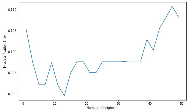
Code : Misclassification error versus k

Python3 1== `

MSE = [1-x for x in cv_scores]

determining the best k

optimal_k = neighbors[MSE.index(min(MSE))] print('The optimal number of neighbors is % d ' % optimal_k)

plot misclassification error versus k

plt.figure(figsize = (10, 6)) plt.plot(neighbors, MSE) plt.xlabel('Number of neighbors') plt.ylabel('Misclassification Error') plt.show()

Output:

The optimal number of neighbors is 13