ML | Breast Cancer Wisconsin Diagnosis using Logistic Regression (original) (raw)

Last Updated : 11 Jul, 2025

Breast Cancer Wisconsin Diagnosis dataset is commonly used in machine learning to classify breast tumors as malignant (cancerous) or benign (non-cancerous) based on features extracted from breast mass images. In this article we will apply **Logistic Regression algorithm for binary classification to predict the nature of breast tumors. It is ideal for such tasks where the goal is to classify data into two categories. We will walk through the steps of preprocessing the data, training the model and evaluating its performance, demonstrating how this model work in early detection and diagnosis of breast cancer.

Implementation of Breast Cancer Detection Using Logistic Regression

Below is the step-by-step implementation:

**1. Loading Libraries

Here we will use**numpy, **pandas, **matplotlib and **scikit learn****.**

Python `

import numpy as np import pandas as pd import matplotlib.pyplot as plt from sklearn.model_selection import train_test_split

`

**2. Loading dataset

You can download dataset from****:** **click here

Python `

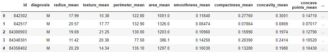
data = pd.read_csv("data.csv") print (data.head)

`

**Output :

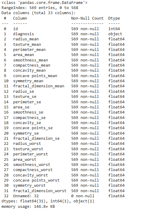
**Getting Information about the dataset.

Python `

data.info()

`

**Output:

3. Processing Dataset

We are dropping columns - 'id' and 'Unnamed: 32' as they have no role in prediction

• data['diagnosis'].map(): Converts the diagnosis column, which contains 'M' (Malignant) and 'B' (Benign) into binary values. 'M' is converted to 1 and 'B' to 0 making it suitable for logistic regression. Python `

data.drop(['Unnamed: 32', 'id'], axis=1, inplace=True) data['diagnosis'] = data['diagnosis'].map({'M': 1, 'B': 0})

`

**Input and Output data

Python `

y = data['diagnosis'].values x_data = data.drop(['diagnosis'], axis=1)

`

**Normalization

Here we will normalize dataset.

• **x_data - x_data.min(): subtracts the minimum value from each value in the dataset shifting the data so that the smallest value becomes 0.
• **x_data.max() - x_data.min(): calculates the range of the data (difference between the maximum and minimum values). Python `

x = (x_data - x_data.min()) / (x_data.max() - x_data.min())

`

**4. Splitting data for training and testing.

• **train_test_split: This function splits your data into two parts one for training your model and another for testing.
• test_size=0.15: 15% of the data will be used for testing and 85% for training.
• **x_train = x_train.T: Transpose ( T ) to ensure that the data has the correct shape for matrix operations during the logistic regression. Python `

from sklearn.model_selection import train_test_split x_train, x_test, y_train, y_test = train_test_split( x, y, test_size = 0.15, random_state = 42)

x_train = x_train.T x_test = x_test.T y_train = y_train.T y_test = y_test.T

print("x train: ", x_train.shape) print("x test: ", x_test.shape) print("y train: ", y_train.shape) print("y test: ", y_test.shape)

`

**Output :

x train: (30, 483) x test: (30, 86) y train: (483,) y test: (86,)

5. Initializing Model Architecture

**Initializing Weight and bias

Python `

def initialize_weights_and_bias(dimension): w = np.random.randn(dimension, 1) * 0.01
b = 0.0 return w, b

`

**Sigmoid Function to calculate z value.

• **sigmoid(): It squashes the input value z between 0 and 1 making it suitable for binary classification. Python `

def sigmoid(z): return 1 / (1 + np.exp(-z))

`

**Forward-Backward Propagation

• np.dot(w.T, x_train): Computes the matrix multiplication of the weights and the input data.
• **cost = (-1/m) * np.sum(y_train * np.log(y_head) + (1 - y_train) * np.log(1 - y_head)): Measures the difference between the predicted probability (y_head) and true label (y_train).
• **derivative_weight = (1/m) * np.dot(x_train, (y_head - y_train).T): This calculates the gradient of the cost with respect to the weights w. It tells us how much we need to change the weights to reduce the cost.
• **derivative_bias = (1/m) * np.sum(y_head - y_train): This computes the gradient of the cost with respect to the bias b. It is simply the average of the difference between predicted probabilities (y_head) and actual labels (y_train). Python `

def forward_backward_propagation(w, b, x_train, y_train): m = x_train.shape[1] z = np.dot(w.T, x_train) + b y_head = sigmoid(z)

cost = (-1/m) * np.sum(y_train * np.log(y_head) + (1 - y_train) * np.log(1 - y_head))

derivative_weight = (1/m) * np.dot(x_train, (y_head - y_train).T)
derivative_bias = (1/m) * np.sum(y_head - y_train)

gradients = {"derivative_weight": derivative_weight, "derivative_bias": derivative_bias}
return cost, gradients

`

**Updating Parameters

• **w -= learning_rate * gradients["derivative_weight"] and **b -= learning_rate * gradients["derivative_bias"]: Weight(w) and Bias(b) are updated by subtracting the gradient scaled by the learning rate. Python `

def update(w, b, x_train, y_train, learning_rate, num_iterations): costs = [] gradients = {} for i in range(num_iterations): cost, grad = forward_backward_propagation(w, b, x_train, y_train) w -= learning_rate * grad["derivative_weight"] b -= learning_rate * grad["derivative_bias"]

    if i % 100 == 0:
        costs.append(cost)
        print(f"Cost after iteration {i}: {cost}")

parameters = {"weight": w, "bias": b}
return parameters, gradients, costs

`

**6. Making Predictions

• np.dot(w.T, x_test): This performs a matrix multiplication between the transposed weights (w.T) and test data (x_test).
• sigmoid(z): Applies the sigmoid activation function to the logits, this function maps the values to the range [0, 1].
• z[0, i] > 0.5: If the probability for the positive class (class 1) is greater than 0.5 then prediction is 1 otherwise it is 0. Python `

def predict(w, b, x_test): m = x_test.shape[1] y_prediction = np.zeros((1, m)) z = sigmoid(np.dot(w.T, x_test) + b)

for i in range(z.shape[1]):
    y_prediction[0, i] = 1 if z[0, i] > 0.5 else 0

return y_prediction

`

**Logistic Regression

• **logistic_regression(x_train, y_train, x_test, y_test, learning_rate=0.01, num_iterations=1000): This line runs the logistic regression model with the given training and test data, a learning rate of 0.01 and 1000 iterations for training. Python `

def logistic_regression(x_train, y_train, x_test, y_test, learning_rate=0.01, num_iterations=1000): dimension = x_train.shape[0] w, b = initialize_weights_and_bias(dimension) parameters, gradients, costs = update(w, b, x_train, y_train, learning_rate, num_iterations)

y_prediction_test = predict(parameters["weight"], parameters["bias"], x_test)
y_prediction_train = predict(parameters["weight"], parameters["bias"], x_train)

print(f"Train accuracy: {100 - np.mean(np.abs(y_prediction_train - y_train)) * 100}%")
print(f"Test accuracy: {100 - np.mean(np.abs(y_prediction_test - y_test)) * 100}%")

logistic_regression(x_train, y_train, x_test, y_test, learning_rate=0.01, num_iterations=1000)

`

**Output :

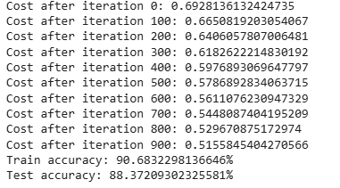
Model Predictions

**We can see that model is working fine as train and test accuracy is similar i.e this model can be used for real world breast cancer detection. After analyzing the dataset, applying logistic regression and evaluating the model's performance we have successfully predicted the diagnosis of breast cancer based on the given features. This demonstrates the effectiveness of machine learning in medical predictions and showcases the power of logistic regression in classification tasks.

**Get the complete notebook here:

Notebook link : **click here.