MiniBatch Gradient Descent with Python (original) (raw)
Mini-Batch Gradient Descent with Python
Last Updated : 12 May, 2026
Gradient Descent is an optimization algorithm used to find optimal model parameters by minimizing the loss through iterative updates in the direction of the steepest descent.
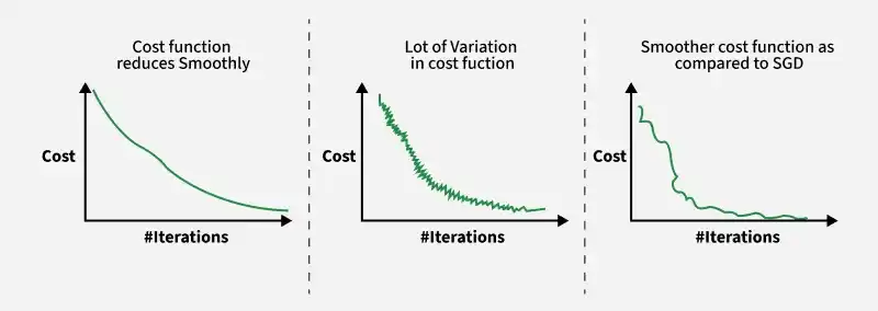
Convergence in BGD, SGD and MBGD
- Updates weights and bias to reduce model error
- Uses gradients of the loss function to guide updates
- Iterative process that improves model performance over time
- Has three main variants: Batch, Stochastic (SGD), and Mini-Batch Gradient Descent
- Each variant differs in speed, stability, and convergence behavior
**Working of Mini-Batch Gradient Descent
Mini-batch gradient descent updates model parameters using small data subsets, balancing the speed of SGD and the stability of batch gradient descent for efficient and stable training.
- Updates parameters using small batches instead of full dataset or single samples
- Faster and more efficient due to parallel processing on GPUs/TPUs
- Converges faster with more frequent updates than batch gradient descent
- Produces smoother convergence compared to stochastic updates
- Introduces slight randomness, helping avoid local minima
- Memory efficient as it does not require loading the entire dataset
**Algorithm:
Let:
- \theta = model parameters
max_iters= number of epochs- \eta = learning rate
For itr=1,2,3,…,max_iters:
- Shuffle the training data. It is optional but often done for better randomness in mini-batch selection.
- Split the dataset into mini-batches of size b.
For each mini-batch (X_{mini}, y_{mini}):
1. Forward Pass on the batch X_mini**:**
Make predictions on the mini-batch
\hat{y} = f(X_{\text{mini}},\ \theta)
Compute error in predictions J(θ) with the current values of the parameters
J(θ)=L(\hat{y},y_{mini})
**2. Backward Pass:
Compute gradient:
\nabla_{\theta} J(\theta) = \frac{\partial J(\theta)}{\partial \theta}
**3. Update parameters:
Gradient descent rule:
\theta = \theta - \eta \nabla_{\theta} J(\theta)
**Python Implementation
Here we will use Mini-Batch Gradient Descent for Linear Regression.
1. Importing Libraries
We begin by importing libraries like NumpyandMatplotlib.pyplot
Python `
import numpy as np import matplotlib.pyplot as plt
`
2. Generating Synthetic 2D Data
Here, we generate 8000 two-dimensional data points sampled from a multivariate normal distribution:
- The data is centered at the point (5.0, 6.0).
- The
covmatrix defines the variance and correlation between the features. A value of0.95indicates a strong positive correlation between the two features. Python `
mean = np.array([5.0, 6.0]) cov = np.array([[1.0, 0.95], [0.95, 1.2]]) data = np.random.multivariate_normal(mean, cov, 8000)
`
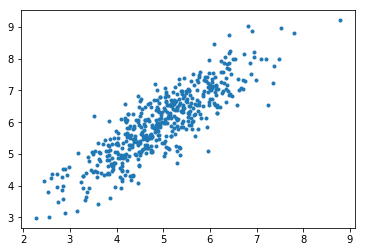
3. Visualizing Generated Data
Python `
plt.scatter(data[:500, 0], data[:500, 1], marker='.') plt.title("Scatter Plot of First 500 Samples") plt.xlabel("Feature 1") plt.ylabel("Feature 2") plt.grid(True) plt.show()
`
**Output:
4. Splitting Data
We split the data into training and testing sets:
- Original data shape:
(8000, 2) - New shape after adding bias:
(8000, 3) - 90% of the data is used for training and 10% for testing. Python `
data = np.hstack((np.ones((data.shape[0], 1)), data))
split_factor = 0.90 split = int(split_factor * data.shape[0])
X_train = data[:split, :-1] y_train = data[:split, -1].reshape((-1, 1)) X_test = data[split:, :-1] y_test = data[split:, -1].reshape((-1, 1))
`
5. Displaying Datasets
Python `
print("Number of examples in training set = %d" % X_train.shape[0]) print("Number of examples in testing set = %d" % X_test.shape[0])
`
**Output:

results
6. Defining Core Functions of Linear Regression
- **Hypothesis(X, theta): Computes the predicted output using the linear model h(X)=X⋅θ
- **Gradient(X, y, theta): Calculates the gradient of the cost function which is used to update model parameters during training.
- **Cost(X, y, theta): Computes the Mean Squared Error (MSE). Python `
def hypothesis(X, theta): return np.dot(X, theta)
def gradient(X, y, theta): h = hypothesis(X, theta) grad = np.dot(X.T, (h - y)) return grad
def cost(X, y, theta): h = hypothesis(X, theta) J = np.dot((h - y).T, (h - y)) / 2 return J[0]
`
7. Creating Mini-Batches for Training
This function divides the dataset into **random mini-batches used during training:
- Combines the feature matrix X and target vector y, then shuffles the data to introduce randomness.
- Splits the shuffled data into batches of size batch_size.
- Each mini-batch is a tuple (X_mini, Y_mini) used for one update step in mini-batch gradient descent.
- Also handles the case where data isn’t evenly divisible by the batch size by including the leftover samples in an extra batch. Python `
def create_mini_batches(X, y, batch_size): mini_batches = [] data = np.hstack((X, y)) np.random.shuffle(data) n_minibatches = data.shape[0] // batch_size for i in range(n_minibatches + 1): mini_batch = data[i * batch_size:(i + 1) * batch_size, :] X_mini = mini_batch[:, :-1] Y_mini = mini_batch[:, -1].reshape((-1, 1)) mini_batches.append((X_mini, Y_mini)) if data.shape[0] % batch_size != 0: mini_batch = data[i * batch_size:] X_mini = mini_batch[:, :-1] Y_mini = mini_batch[:, -1].reshape((-1, 1)) mini_batches.append((X_mini, Y_mini)) return mini_batches
`
8. Mini-Batch Gradient Descent Function
This function performs mini-batch gradient descent to train the linear regression model:
- **Initialization: Weights
thetaare initialized to zeros and an empty listerror_listtracks the cost over time. - **Training Loop: For a fixed number of iterations (
max_iters), the dataset is divided into mini-batches. - **Each mini-batch: computes the gradient, updates
thetato reduce cost and records the current error for tracking training progress. Python `
def gradientDescent(X, y, learning_rate=0.001, batch_size=32): theta = np.zeros((X.shape[1], 1)) error_list = [] max_iters = 3
for itr in range(max_iters):
    mini_batches = create_mini_batches(X, y, batch_size)
    for X_mini, y_mini in mini_batches:
        theta = theta - learning_rate * gradient(X_mini, y_mini, theta)
        error_list.append(cost(X_mini, y_mini, theta))

return theta, error_list
`
9. Training and Visualization
The model is trained using gradientDescent() on the training data. After training:
- theta[0] is the bias term (intercept).
- theta[1:] contains the feature weights (coefficients).
- The plot shows how the cost decreases as the model learns, showing convergence of the algorithm.
This provides a visual and quantitative insight into how well the mini-batch gradient descent is optimizing the regression model.
Python `
theta, error_list = gradientDescent(X_train, y_train) print("Bias = ", theta[0]) print("Coefficients = ", theta[1:])
plt.plot(error_list) plt.xlabel("Number of iterations") plt.ylabel("Cost") plt.show()
`
**Output:

Mini-Batch over Regression model
10. Final Prediction and Evaluation
**Prediction: The hypothesis() function is used to compute predicted values for the test set.
**Visualization:
- A scatter plot shows actual test values.
- A line plot overlays the predicted values, helping to visually assess model performance.
**Evaluation:
- Computes Mean Absolute Error (MAE) to measure average prediction deviation.
- A lower MAE indicates better accuracy of the model. Python `
y_pred = hypothesis(X_test, theta)
plt.scatter(X_test[:, 1], y_test, marker='.', label='Actual') plt.plot(X_test[:, 1], y_pred, color='orange', label='Predicted') plt.xlabel("Feature 1") plt.ylabel("Target") plt.title("Model Predictions vs Actual Values") plt.legend() plt.grid(True) plt.show()
error = np.sum(np.abs(y_test - y_pred)) / y_test.shape[0] print("Mean Absolute Error =", error)
`
**Output:

Model prediction and Actual values
Batch vs Stochastic vs Mini-Batch Gradient Descent.
| **Type | **Update Strategy | **Speed and Efficiency | **Noise in Updates | **Memory Usage |
|---|---|---|---|---|
| **Batch Gradient Descent | Uses entire dataset for each update | Slow, high computation cost | Smooth and stable | High (needs full dataset in memory) |
| **Stochastic Gradient Descent (SGD) | Updates using one sample at a time | Fast updates but less efficient overall | Highly noisy updates | Low |
| **Mini-Batch Gradient Descent | Uses small batches of datatraining examples | Fast and efficient (supports vectorization) | Moderate noise—dependent on batch size | Moderate |