Multiple Linear Regression with Backward Elimination (original) (raw)
Last Updated : 12 Jul, 2025
**Multiple Linear Regression (MLR) is a statistical technique used to model the relationship between a dependent variable and multiple independent variables. However, not all variables significantly contribute to the model. **Backward Elimination technique helps in selecting only the most significant predictors, improving model efficiency and interpretability.
Understanding Multiple Linear Regression
Multiple Linear Regression (MLR) extends simple linear regression by incorporating multiple independent variables to predict a dependent variable.
The general equation is:
y = b_0 + b_1x_1 + b_2x_2 + ... + b_nx_n + \epsilon
where:
- y is the dependent variable (target outcome),
- x_1, x_2 ,..., x_n are independent variables (predictors),
- b_0, b_1 , ..., b_n are regression coefficients,
- ϵ is the error term, accounting for variability not explained by the predictors.
The goal is to estimate the coefficients that best fit the given data while minimizing errors.
What is Backward Elimination?
**Backward Elimination is a stepwise **feature selectiontechnique used in MLR to identify and remove the least significant features. It systematically eliminates variables based on their statistical significance, improving model accuracy and interpretability.
Steps in Backward Elimination
Backward Elimination follows these systematic steps:
- **Select a significance level (SL): Commonly set to **0.05.
- **Fit the model with all independent variables.
- **Identify the predictor with the highest P-value:
- If P-value > SL, proceed to step 4.
- Otherwise, retain the predictor and finalize the model.
- **Remove the predictor with the highest P-value.
- **Recalculate the model without the removed predictor.
- **Repeat steps 3-5 until all remaining variables have P-values below SL.
Example Use Case: Predicting Sales Based on Advertising Budget
We will use the ****"Advertising Dataset"** to predict sales based on different advertising budgets. The dataset contains information on **TV, Radio, and Newspaper advertising budgets and their impact on sales. Our goal is to determine which advertising channel has the most significant effect on sales.
Step 1: Import Libraries
First, import the necessary libraries: NumPy, Pandas, and Statsmodels.
C++ `
import numpy as np import pandas as pd import statsmodels.api as sm
`
Step 2: Load the Dataset
Let's load the dataset and divide the independent and dependent variable. You can download the dataset from here: **Advertising Dataset
C++ `
dataset = pd.read_csv('advertising.csv')
Independent variables
X = dataset.iloc[:, :-1].values
Dependent variable
y = dataset.iloc[:, -1].values
`
**Step 3: Add a Column of Ones (Intercept Term)
Now, let's add a column of ones to the independent variables matrix (X) t o account for the intercept term in the regression model.
**Why to perform this step?
Unlike some machine learning libraries (e.g., scikit-learn), statsmodels does not automatically include an intercept term in the model. You must explicitly add it.
- **np.ones((X.shape[0], 1)): Creates a column vector of ones with the same number of rows as X.
- ****.astype(int):** Ensures the column of ones is of integer type.
- **np.append(..., axis=1): Appends the column of ones as the first column of X. C++ `
X = np.append(arr=np.ones((X.shape[0], 1)).astype(int), values=X, axis=1)
`
**Step 4: Fit the Model & Perform Backward Elimination
Now, we will implement backward elimination algorithm to iteratively remove insignificant predictors from the model.
- It starts with a full model (all predictors included).
- At each step, it removes the predictor with the highest p-value (if the p-value exceeds a specified significance level, e.g., 0.05) using **max_p_value > significance_level and **np.delete(X, max_p_index, axis=1)
- The process stops when all remaining predictors have p-values below the significance level. C++ `
def backward_elimination(X, y, significance_level=0.05): num_vars = X.shape[1] for i in range(num_vars): regressor_OLS = sm.OLS(y, X).fit() # Fit model using Ordinary Least Squares (OLS) max_p_value = max(regressor_OLS.pvalues) # Get the highest p-value if max_p_value > significance_level: # If p-value is greater than the threshold, remove that predictor max_p_index = np.argmax(regressor_OLS.pvalues) X = np.delete(X, max_p_index, axis=1) else: break # Stop when all p-values are below the significance level return X, regressor_OLS
X_optimized, final_model = backward_elimination(X, y)
`
**Step 5: View Final Model Summary
Once backward elimination is complete, detailed summary of the final regression model is displayed.
C++ `
print(final_model.summary())
`
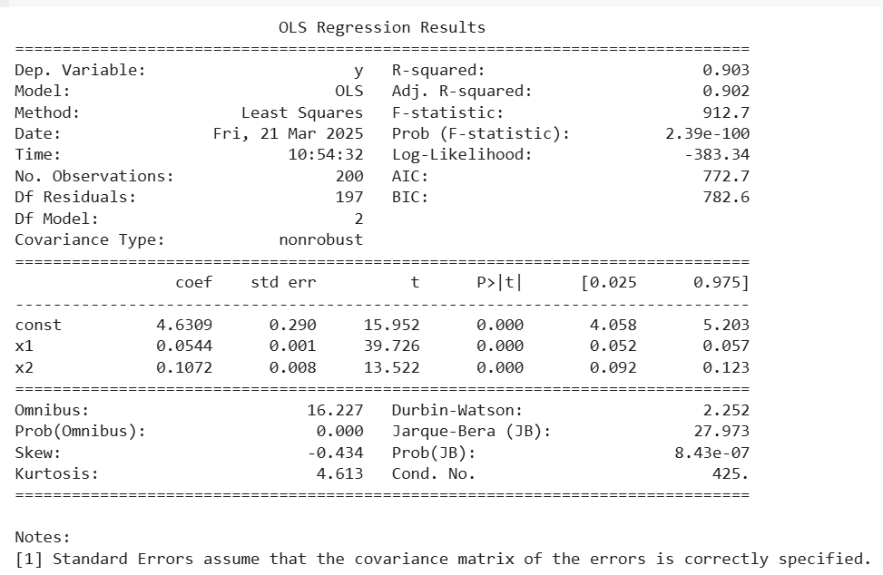
- In this OLS results, all predictors (x1 and x2) have **p-values of 0.000, which are **less than 0.05, meaning they are **statistically significant and should be retained.
- The **Adjusted R² value (0.902) confirms that the model performs well even after accounting for the number of predictors.
- Since all predictors meet the statistical significance criterion, **backward elimination stops here, and the final model is selected.
**Forward Selection vs Backward Elimination
Both **Forward Selection and **Backward Elimination are stepwise regression methods used for feature selection. Here’s a comparison:
| Feature | Forward Selection | Backward Elimination |
|---|---|---|
| Approach | Starts with **no variables and adds the most significant one iteratively. | Starts with **all variables and removes the least significant one iteratively. |
| Initial Model | Begins with only the intercept (constant). | Begins with all independent variables. |
| Process | Adds variables one by one based on the lowest p-value. | Removes variables one by one based on the highest p-value. |
| Stopping Criterion | Stops when no remaining variable has **p-value < 0.05. | Stops when all remaining variables have **p-value < 0.05. |
| When to Use? | When the dataset has many independent variables (unknown importance). | When we want to simplify a full model with all features. |
| Accuracy | May not always find the best model. | Often leads to a more accurate and simplified model. |