Normal Equation in Linear Regression (original) (raw)

Last Updated : 11 Jul, 2025

Linear regression is a popular method for understanding how different factors (independent variables) affect an outcome (dependent variable. At its core, linear regression aims to find the best-fitting line that minimizes the error between observed data points and predicted values. One efficient method to achieve this is through the use of the normal equation. In this article, we will understand in-depth into the details of the normal equation, its mathematical derivation, implementation, and comparison with other optimization methods like gradient descent.

Linear Regression using Normal Equation

Table of Content

• Understanding Normal Equation in Linear Regression
• Mathematical Derivation: Behind the Equation
• Python implementation of Normal Equation
• The Normal Equation vs Gradient Descent

Understanding Normal Equation in Linear Regression

The normal equation is a mathematical formula that provides a straightforward way to calculate the coefficients (β\betaβ) in linear regression. Instead of using trial-and-error or iterative methods, the normal equation allows us to find the best coefficients directly. The formula for the normal equation is:

Normal equation formula

In the above equation,

**θ: hypothesis parameters that define it the best.
**X: Input feature value of each instance.
**Y: Output value of each instance.

The Normal Equation leverages the **power of matrix algebra to efficiently handle multiple independent variables in linear regression. By organizing the data into matrices, the equation helps in linear transformations and calculations that simplify the process of finding the best-fitting coefficients.

One of the significant advantages of the Normal Equation is its computational efficiency, especially for small to medium-sized datasets. **Unlike iterative methods such as gradient descent, which require multiple passes over the data to converge on the optimal coefficients, the Normal Equation calculates all coefficients in one shot. This results in faster computations and a straightforward implementation when the dataset size is manageable. However, it is essential to note that as the number of features or data points increases significantly, the computation of the inverse of the matrix can become computationally expensive, leading to potential issues with numerical stability.

Mathematical Derivation: Behind the Equation

To derive the Normal Equation, we start with the least squares minimization problem, aiming to minimize the sum of squared residuals:

J(\theta) = \frac{1}{2} \sum_{i=1}^{n} (y_i - (\theta_0 + \theta_1 x_i))^2

where:

• n is the number of observations,
• y_i is the i^{th} observed value,
• x_i is the i^{th} feature value.

Explanation of the Hypothesis Function

Given the hypothesis function,

h(\theta) = \theta_0 x_0 + \theta_1 x_1 + \theta_2 x_2 + \theta_3 x_3 + \ldots + \theta_n x_n

where:

• **n: the no. of features in the data set.
• **x 0 : 1 (for vector multiplication)

Notice that this is a dot product between θ and x values. So for the convenience to solve we can write it as:

h(\theta) = \theta^T X

Formulating the Cost Function

Next, we express the cost function. For simplicity, we omit the 1/2m​ factor since it doesn’t affect the optimization when using the normal equation.

We have ignored here as it will not make any difference in the working. It was used for mathematical convenience while calculating gradient descent. But it is no more needed here.

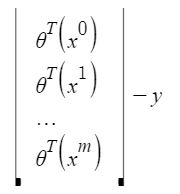
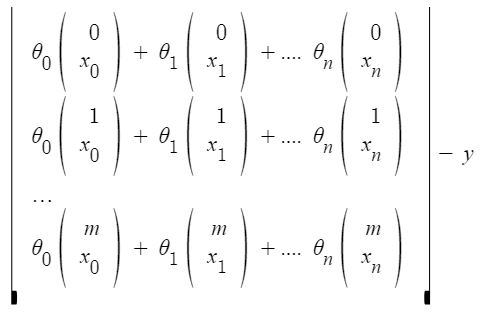
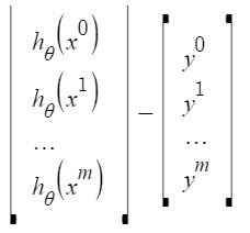
Each feature value in the x^{i}_j****:** i.e the value of j^{ij} feature in i^{th} training example. The difference between predicted values and actual values (the residuals) can further be reduced to:

X\theta - y

To compute the cost, we need to square these residuals. However, squaring a vector or matrix requires multiplying it by its transpose. Thus, we can express the cost function as:

(X\theta - y)^T(X\theta - y)

Therefore, the cost function is

Cost = (X\theta - y)^T(X\theta - y)

Calculating the Value of θ using the partial derivative of the Normal Equation

To find the values of \theta_0 and \theta_1 that minimizeJ(\theta), we compute the partial derivatives with respect to \theta_0 and \theta_1 and set them to zero.

Let's take a partial derivative of the cost function with respect to the parameter theta. Note that in partial derivative we treat all variables except the parameter theta as constant.

\frac{\partial J}{\partial \theta} = \frac{\partial}{\partial \theta} \left( (X\theta - y)^T(X\theta - y) \right)

\frac{\partial J}{\partial \theta} = 2X^T(X\theta - y)

We know to find the optimum value of any partial derivative equation we have to equate it to 0.

Cost(\theta) = 0

2X^TX\theta - X^Ty = 0

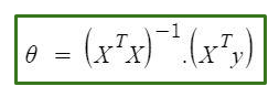
To find the optimal values of θ, we solve the normal equations derived from the cost function. We begin with the equation:

2X^TX\theta = X^Ty

To isolate θ, we multiply both sides of the equation by the inverse of 2X^{⊺}X, leads to the normal equation:

\theta = (X^\intercal X)^{-1}X^\intercal y

This formula represents the solution for θ in terms of the design matrix X and the vector of observed values y. Here:

• X is the design matrix, which contains the input features (including a column of ones for the intercept).
• y is the vector of observed output values.
• X^T is the transpose of the matrix X.

Thus, the final expression for θ is given by:

Normal Equation

This equation enables us to compute the optimal parameters for linear regression directly using matrix operations.

Python implementation of Normal Equation

We can implement this normal equation using Python programming language. We will create a synthetic dataset using sklearn having only one feature. Also, we will use numpy for mathematical computation like for getting the matrix to transform and inverse of the dataset. Also, we will use try and except block in our function so that in case if our input data matrix is singular our function will not be throwing an error.

Python `

import numpy as np from sklearn.datasets import make_regression

Create data set.

X, y = make_regression(n_samples=100, n_features=1, n_informative=1, noise=10, random_state=10)

def linear_regression_normal_equation(X, y): X_transpose = np.transpose(X) X_transpose_X = np.dot(X_transpose, X) X_transpose_y = np.dot(X_transpose, y)

try:
    theta = np.linalg.solve(X_transpose_X, X_transpose_y)
    return theta
except np.linalg.LinAlgError:
    return None

Add a column of ones to X for the intercept term

X_with_intercept = np.c_[np.ones((X.shape[0], 1)), X]

theta = linear_regression_normal_equation(X_with_intercept, y) if theta is not None: print(theta) else: print("Unable to compute theta. The matrix X_transpose_X is singular.")

`

**Output:

[ 0.52804151 30.65896337]

To Predict on New Test Data Instances

Since we have trained our model and have found parameters that give us the lowest error. We can use this parameter to predict on new unseen test data.

Python `

def predict(X, theta): predictions = np.dot(X, theta) return predictions

Input features for testing

X_test = np.array([[1], [4]]) X_test_with_intercept = np.c_[np.ones((X_test.shape[0], 1)), X_test] predictions = predict(X_test_with_intercept, theta) print("Predictions:", predictions)

Plotting the results

plt.scatter(X, y, color='blue', label='Data Points') # Plot the original data points plt.plot(X, predict(X_with_intercept, theta), color='red', label='Regression Line') # Plot the regression line plt.scatter(X_test, predictions, color='green', marker='x', label='Predictions') # Plot the predictions plt.title('Linear Regression using Normal Equation') plt.xlabel('Feature (X)') plt.ylabel('Target (y)') plt.legend() plt.grid() plt.show()

`

**Output:

Predictions: [ 31.18700488 123.16389501]

Linear Regression using Normal Equation

The Normal Equation vs Gradient Descent

These are the two primary methods for estimating the coefficients (parameters) in Linear Regression Model. Each method has its unique advantages and considerations, making them suitable for different scenarios. Let's see a detailed comparison between these two approaches. The normal equation provides an analytical solution, computing the optimal parameters in a single step. Gradient descent uses an iterative approach, updating the parameters until convergence.

The Normal Equation provides a closed-form solution to linear regression, allowing for the computation of optimal coefficients in one step.

• This method is efficient for small to medium-sized datasets because it relies on straightforward matrix operations.
• However, its dependence on matrix inversion can become computationally expensive with large datasets.
• Additionally, the Normal Equation does not require hyperparameter tuning, making its implementation simpler.

In contrast, **Gradient Descent is an iterative optimization algorithm that adjusts the coefficients incrementally based on the gradient of the cost function.

• This method is particularly effective for large datasets, as it can process data points one at a time or in mini-batches, thereby reducing memory requirements.
• While Gradient Descent may take longer to converge compared to the Normal Equation, its performance can be significantly influenced by the choice of learning rate, which necessitates some degree of hyperparameter tuning.
• Furthermore, there are several variants of Gradient Descent, including stochastic and mini-batch methods, that can improve convergence speed and model generalization.

In summary, the choice between the normal equation and gradient descent often depends on the characteristics of the dataset and the problem at hand:

• **Use the Normal Equation:
  • When working with smaller datasets or when a quick solution is needed without iterative tuning.
  • When simplicity and directness are prioritized.
• **Use Gradient Descent:
  • When handling large datasets or when the feature set is extensive, which could make matrix inversion computationally prohibitive.
  • When a more flexible approach is needed, especially if the model complexity increases or if you're working with online learning scenarios.

Both methods are fundamental to understanding linear regression, and knowing when to use each can significantly impact the efficiency and effectiveness of your machine learning solutions.