SemiSupervised Learning in ML (original) (raw)

Semi-Supervised Learning in ML

Last Updated : 30 Apr, 2026

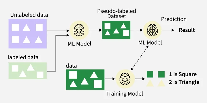
Semi-supervised learning is a distinct machine learning approach that uses a small amount of labeled data along with a large amount of unlabeled data to improve model performance. The goal is to learn a function that accurately predicts outputs based on inputs, similar to supervised learning, but with much less labelled data.

Semi-Supervised Learning

Semi-supervised learning is particularly valuable when acquiring labelled data is expensive or time-consuming, yet unlabelled data is plentiful and easy to collect.

• **Supervised learning: Similar to a student being taught concepts by a teacher both in class and at home.
• **Unsupervised learning: Like a student figuring out concepts independently without instruction like a math problem.
• **Semi-supervised learning: A mix where the teacher provides some concepts in class and the student practices with homework assignments based on those concepts.

Working of Semi-Supervised Learning

• **Self-Training: The model is first trained on labeled data. It then predicts labels for unlabeled data, adding high-confidence predictions to the labeled set iteratively to refine the model.
• **Co-Training: Two models are trained on different feature subsets of the data. Each model labels unlabeled data for the other, enabling them to learn from complementary views.
• **Multi-View Training: A variation of co-training where models train on different data representations (e.g., images and text) to predict the same output.
• **Graph-Based Models: Data is represented as a graph with nodes (data points) and edges (similarities). Labels are propagated from labeled nodes to unlabeled ones based on graph connectivity.

Let's see an example to understand better.

Step 1: Importing Libraries and Loading Data

We will import the necessary libraries such as numpy, matplotlib and sklearn. We will load IRIS Dataset.

Python `

import numpy as np import matplotlib.pyplot as plt from sklearn import datasets from sklearn.semi_supervised import LabelPropagation from sklearn.metrics import accuracy_score

iris = datasets.load_iris() X = iris.data[:, :2] y = iris.target

`

Step 2: Semi-Supervised Setup (Mask Labels)

We will setup the semi-supervised working,

• labels is what we pass to the algorithm (contains -1 for unlabeled).
• mask is a boolean array indicating which points keep their labels.
• labels[~mask] = -1 is a scikit-learn convention where -1 represents unlabeled data.
• Print helps readers see how many labels remain (important when describing experiments). Python `

labels = np.copy(y) rng = np.random.RandomState(42) mask = rng.rand(len(y)) < 0.1 labels[mask] = -1 print(f"Labeled: {np.sum(mask)}, Unlabeled: {np.sum(mask)}")

`

Step 3: Train a Graph-Based Model (Label Propagation)

We will train a graph-based model,

• LabelPropagation() builds a graph on X (similarities) and propagates labels from labeled nodes to unlabeled ones.
• fit(X, labels) performs the label diffusion — no separate .predict() needed for transduction. Python `

model = LabelPropagation() model.fit(X, labels)

`

Step 4: Get Transduced Labels and Evaluate

Labels are assigned to all points,

• model.transduction_ gives the inferred labels for every sample (including previously unlabeled).
• Evaluate both on the small originally-labeled subset (y[mask]) and on the true labels (y) to show how well propagation recovered the full labeling.
• accuracy_score is a simple, interpretable metric. Python `

y_pred = model.transduction_ acc_labeled = accuracy_score(y[mask], y_pred[mask]) acc_overall = accuracy_score(y, y_pred) print(f"Acc (on original labeled subset): {acc_labeled:.3f}") print(f"Acc (overall after propagation): {acc_overall:.3f}")

`

**Output:

Labeled samples: 18, Unlabeled samples: 132
Accuracy on labeled data: 1.00
Overall accuracy after label propagation: 0.71

Step 5: Visualize

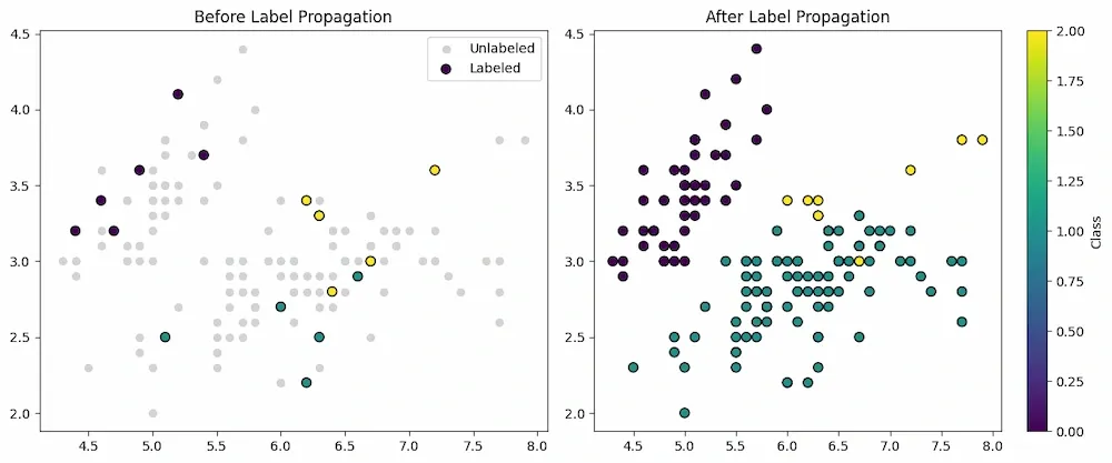
We will visualize results:

• Left plot shows the few labeled examples (colored) against unlabeled (gray).
• Right plot shows model’s assigned labels for every point after propagation.
• Removing edgecolor avoids common scatter warnings. Python `

fig, ax = plt.subplots(1, 2, figsize=(12, 4))

ax[0].scatter(X[:, 0], X[:, 1], c='lightgray', s=30) ax[0].scatter(X[mask, 0], X[mask, 1], c=y[mask], cmap='viridis', s=60) ax[0].set_title("Before propagation — few labels")

ax[1].scatter(X[:, 0], X[:, 1], c=y_pred, cmap='viridis', s=60) ax[1].set_title("After propagation — all labeled")

plt.tight_layout() plt.show()

`

**Output:

Result

As we can see in the result that the model was able to classify images into the categories or labels after successful operations of semi-supervised learning.

When to Use

• When labeled data is scarce or costly, such as medical imaging requiring expert annotation.
• When large volumes of unlabeled data exist, like social media or web content.
• For unstructured data types (text, images, audio) where labeling is difficult.
• When classes are rare and labeled examples few, improving class recognition.
• When purely supervised or unsupervised methods are insufficient.

Applications

• **Face Recognition: Enhancing accuracy by learning from limited labeled face images plus many unlabeled ones using graph-based methods.
• **Handwritten Text Recognition: Adapting models to diverse handwriting styles through generative models.
• **Speech Recognition: Improving transcription quality by using unlabeled speech data with CNNs and other techniques.
• **Security: Google uses semi-supervised learning for anomaly detection in network traffic and malware detection.
• **Finance: PayPal applies it for fraud detection and creditworthiness assessment using transaction data.

Advantages

• **Better Generalization: Utilizes both labeled and unlabeled data to capture the whole data structure, improving prediction robustness.
• **Cost Efficient: Reduces dependency on costly manual labeling by exploiting unlabeled data.
• **Flexible and Robust: Handles different data types and sources, adapting well to changing data distributions.
• **Improved Clustering: Refines clusters by leveraging unlabeled data, yielding better class separation.
• **Handling Rare Classes: Enhances learning for underrepresented classes where labeled examples are minimal.

Limitations

• **Model Complexity: Requires careful choice of architecture and hyperparameters, which may require extensive tuning.
• **Noisy Data: Unlabeled data may contain errors or irrelevant information, risking degraded model performance.
• **Assumption Sensitivity: Relies on assumptions such as data consistency and clusterability, which may not hold in all cases.
• **Evaluation Challenge: Assessing performance is difficult due to limited labeled data and varied quality of unlabeled data.