Naive Bayes Scratch Implementation using Python (original) (raw)

Last Updated : 24 Mar, 2026

Naive Bayes is a probabilistic machine learning algorithms based on the Bayes Theorem. It is popular method for classification applications such as spam filtering and text classification.

Naive-Bayes

Naive Bayes Working Pipeline

Here we are implementing a Naive Bayes Algorithm from Scratch in Python using Gaussian distributions. It performs all the necessary steps from data preparation and model training to testing and evaluation.

1. Importing Libraries

Importing necessary libraries:

**math: for mathematical operations
**random: for random number generation
**pandas: for data manipulation
**numpy: for scientific computing Python `

import math import random import pandas as pd import numpy as np

2. Encoding Class

The **encode_class function converts class labels in the dataset into numeric values. It assigns a unique numeric identifier to each class.

Python `

def encode_class(mydata): classes = [] for i in range(len(mydata)): if mydata[i][-1] not in classes: classes.append(mydata[i][-1]) for i in range(len(classes)): for j in range(len(mydata)): if mydata[j][-1] == classes[i]: mydata[j][-1] = i return mydata

3. Splitting the Data

The **splitting function is used to split the dataset into training and testing sets based on the given ratio.

Python `

def splitting(mydata, ratio): train_num = int(len(mydata) * ratio) train = [] test = list(mydata)

while len(train) < train_num:
    index = random.randrange(len(test))
    train.append(test.pop(index))
return train, test

4. Grouping Data by Class

The **groupUnderClass function takes the data and returns a dictionary where each key is a class label and the value is a list of data points belonging to that class.

Python `

def groupUnderClass(mydata): data_dict = {} for i in range(len(mydata)): if mydata[i][-1] not in data_dict: data_dict[mydata[i][-1]] = [] data_dict[mydata[i][-1]].append(mydata[i]) return data_dict

5. Calculating Mean and Standard Deviation for Class

The **MeanAndStdDev function takes a list of numbers and calculates the mean and standard deviation.
The **MeanAndStdDevForClass function takes the data and returns a dictionary where each key is a class label and the value is a list of lists, where each inner list contains the mean and standard deviation for each attribute of the class. Python `

def MeanAndStdDev(numbers): avg = np.mean(numbers) stddev = np.std(numbers) return avg, stddev

def MeanAndStdDevForClass(mydata): info = {} data_dict = groupUnderClass(mydata) for classValue, instances in data_dict.items(): info[classValue] = [MeanAndStdDev(attribute) for attribute in zip(*instances)] return info

6. Calculating Gaussian and Class Probabilities

The **calculateGaussianProbability function takes a value, mean and standard deviation and calculates the probability of the value occurring under a Gaussian distribution with that mean and standard deviation.
The **calculateClassProbabilities function takes the information dictionary and a test data point as arguments. It iterates through each class and calculates the probability of the test data point belonging to that class based on the mean and standard deviation of each attribute for that class. Python `

def calculateGaussianProbability(x, mean, stdev): epsilon = 1e-10 expo = math.exp(-(math.pow(x - mean, 2) / (2 * math.pow(stdev + epsilon, 2)))) return (1 / (math.sqrt(2 * math.pi) * (stdev + epsilon))) * expo

def calculateClassProbabilities(info, test): probabilities = {} for classValue, classSummaries in info.items(): probabilities[classValue] = 1 for i in range(len(classSummaries)): mean, std_dev = classSummaries[i] x = test[i] probabilities[classValue] *= calculateGaussianProbability(x, mean, std_dev) return probabilities

7. Predicting for Test Set

The **predict function takes the information dictionary and a test data point as arguments. It calculates the class probabilities and returns the class with the highest probability.
The **getPredictions function takes the information dictionary and the test set as arguments. It iterates through each test data point and predicts its class using the predict function. Python `

def predict(info, test): probabilities = calculateClassProbabilities(info, test) bestLabel = max(probabilities, key=probabilities.get) return bestLabel

def getPredictions(info, test): predictions = [predict(info, instance) for instance in test] return predictions

8. Calculating Accuracy

The **accuracy_rate function takes the test set and the predictions as arguments. It compares the predicted classes with the actual classes and calculates the percentage of correctly predicted data points.

Python `

def accuracy_rate(test, predictions): correct = sum(1 for i in range(len(test)) if test[i][-1] == predictions[i]) return (correct / float(len(test))) * 100.0

9. Loading and Preprocessing Data

The code then loads the data from a CSV file using pandas and converts it into a list of lists. It then encodes the class labels and converts all attributes to floating-point numbers.

Dataset we are using is of diabetes patients and can be downloaded from here.

Python `

filename = 'diabetes.csv' df = pd.read_csv(filename, comment='#') mydata = df.values.tolist()

mydata = encode_class(mydata) for i in range(len(mydata)): for j in range(len(mydata[i]) - 1): mydata[i][j] = float(mydata[i][j])

10. Splitting Data into Training and Testing Sets

The code splits the data into training and testing sets using a specified ratio. It then trains the model by calculating the mean and standard deviation for each attribute in each class.

Python `

ratio = 0.7 train_data, test_data = splitting(mydata, ratio)

print('Total number of examples:', len(mydata)) print('Training examples:', len(train_data)) print('Test examples:', len(test_data))

**Output:

Total number of examples: 1000
Training examples: 700
Test examples: 300

11. Training and Testing the Model

Calculate mean and standard deviation for each attribute within each class for the training set. Finally, it tests the model on the test set and calculates the accuracy.

Python `

info = MeanAndStdDevForClass(train_data)

predictions = getPredictions(info, test_data) accuracy = accuracy_rate(test_data, predictions) print('Accuracy of the model:', accuracy)

**Output:

Accuracy of the model: 100.0

12. Evaluating Model

We will plot different types of visualizations for evaluation:

**1. Confusion Matrix

The confusion matrix summarizes prediction results by showing true positives, false positives, true negatives and false negatives. It helps visualize how well the classifier distinguishes between different classes.

Python `

from sklearn.metrics import confusion_matrix, ConfusionMatrixDisplay

y_true = [row[-1] for row in test_data] y_pred = predictions

cm = confusion_matrix(y_true, y_pred) disp = ConfusionMatrixDisplay(confusion_matrix=cm) disp.plot(cmap='Blues')

**Output:

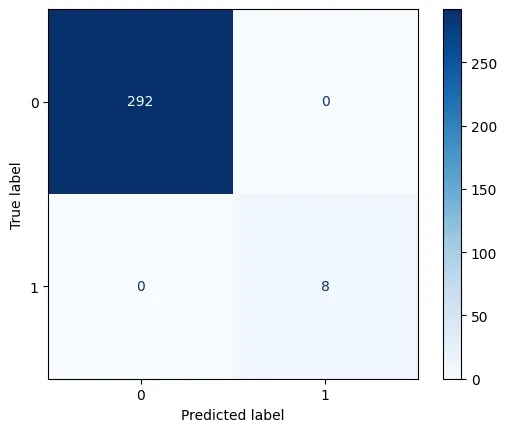
Confusion Matrix

**2. Precision, Recall and F1 score

The F1 score is the harmonic mean of precision and recall, balancing both metrics into a single value. It’s useful when the class distribution is imbalanced or when false positives and false negatives are costly.

Python `

import matplotlib.pyplot as plt from sklearn.metrics import precision_score, recall_score, f1_score

actual = [0, 1, 1, 0, 1, 0, 1, 1] predicted = [0, 1, 0, 0, 1, 0, 1, 0]

precision = precision_score(actual, predicted) recall = recall_score(actual, predicted) f1 = f1_score(actual, predicted)

metrics = ['Precision', 'Recall', 'F1 Score'] values = [precision, recall, f1]

plt.figure(figsize=(6, 4)) plt.bar(metrics, values, color=['skyblue', 'lightgreen', 'salmon']) plt.ylim(0, 1) plt.title('Precision, Recall, and F1 Score') plt.ylabel('Score') for i, v in enumerate(values): plt.text(i, v + 0.02, f"{v:.2f}", ha='center', fontweight='bold')

plt.show()

**Output:

bayes_f1

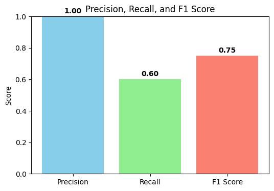
Precision, Recall and F1 Score

You can download the complete source code from here.

Naive Bayes proves to be an efficient and simple algorithm that works well for classification tasks. It is easy to understand since it is based on Bayes' theorem and is simple to use and analyze.