Natural Disaster Prediction in R (original) (raw)

Last Updated : 23 Jul, 2025

Natural disasters are major events that can cause serious harm to people and property. Thanks to modern technology, we can now predict these events more accurately. This article explains how to use the R programming language to analyze data on natural disasters.

**What are Natural Disaster Prediction Models?

Natural Disaster Prediction models are tools or methods used to forecast future events or outcomes based on historical data. By analyzing patterns and trends in past information, these models help us make educated guesses about what might happen next, whether it's predicting the weather, stock prices, or the likelihood of a natural disaster.

**Building a Prediction Model in R

To build a prediction model in R, several key steps are essential to ensure the data is ready for analysis and that the model created is effective. Here's how the overall process works -

1. **Load the Data: Start by bringing your dataset into R. This sets up your project and provides the data you’ll work with.
2. **Analyze the Data: Look at the dataset to understand what’s inside. Get familiar with the data and how it’s organized.
3. **Prepare the Data: Clean and organize the data to make it ready for analysis. Fix any missing values and adjust the data as needed.
4. **Build the Model: Use R’s tools to create your prediction model. Choose the right methods and set them up to analyze the data and find patterns.
5. **Check the Model: Test the model with some of the data to see how well it works. Make sure it’s predicting accurately.
6. **Make Predictions: Use the model to forecast future natural disasters based on the patterns you’ve found.

Understanding Natural Disaster Dataset

The natural disaster dataset provides detailed information about different types of natural disasters, such as earthquakes, hurricanes, and floods. Each record in the dataset has a unique ID and includes the type of disaster, the date it happened, and the exact location where it occurred, with details like latitude and longitude.

For events like earthquakes, the dataset includes the magnitude and depth, while for hurricanes, it provides wind speed and rainfall data. The dataset also records environmental conditions like temperature and humidity at the time of the disaster. Additionally, it includes data on how often similar disasters have occurred in the past, helping to understand patterns and predict future events.

Dataset link : NaturalDisaster

Now we implement stepwise to build the prediction model stepwise in R programing Language.

Step 1: Load the required libaries and dataset

• First load the required libaries and these libraries provide functions for data visualization, manipulation, building prediction models, and creating interactive maps.
• Next read the dataset from a CSV file into an R dataframe.
• Display the first few rows of the dataset to understand its structure and contents. R `

Load necessary libraries

library(ggplot2) library(dplyr) library(randomForest) library(leaflet) library(caret) # Added for cross-validation library(leaflet) # Load the leaflet package

Load the dataset

data <- read.csv("natural_disaster_dataset.csv") head(data)

`

**Output:

ID Disaster_Type Date Location Latitude Longitude Magnitude
1 1 Wildfire 2021-09-05 Joyceshire 15.50625 158.23697 NA
2 2 Wildfire 2021-08-20 West Glenn 39.61520 -113.39889 NA
3 3 Earthquake 2024-02-08 Lake Taylor 32.63846 -117.50888 6.1
4 4 Flood 2022-06-24 West Samantha -26.39599 167.67467 NA
5 5 Wildfire 2023-09-05 Whiteville 74.94508 -50.26314 NA
6 6 Wildfire 2020-11-17 Lorettaland 71.90164 112.23947 NA
Depth Wind_Speed Rainfall Temperature Humidity Historical_Frequency
1 NA NA NA -11.8 24.7 17
2 NA NA NA -19.9 97.8 7
3 677.1 NA NA -28.6 94.2 5
4 NA NA 321.6 42.4 73.9 14
5 NA NA NA 33.1 98.2 6
6 NA NA NA -4.9 99.3 18

Step 2: **Handling Missing Values

• Replaced missing values in numeric columns with the median of the respective column.
• Converted the Date column to the Date format.
• Converted the Disaster_Type column to a factor (categorical variable).
• Ensure that the data types are appropriate for analysis and modeling.
• Address missing data to ensure the model can train without issues related to incomplete data. R `

Step 2: Handle Missing Values

data_cleaned <- data %>% mutate(across(where(is.numeric), ~ ifelse(is.na(.), median(., na.rm = TRUE), .)))

Convert Data Types

data_cleaned$Date <- as.Date(data_cleaned$Date, format="%Y-%m-%d") data_cleaned$Disaster_Type <- as.factor(data_cleaned$Disaster_Type)

`

Step 3: Perform **Exploratory Data Analysis (EDA)

EDA helps in understanding patterns and insights from the data. Visualize different aspects to gain a better understanding.

Plot the Distribution of Disaster Types

Display the distribution of different types of natural disasters.

R `

ggplot(data_cleaned, aes(x = Disaster_Type)) + geom_bar(fill = "pink") + theme_minimal() + labs(title = "Distribution of Disaster Types", x = "Disaster Type", y = "Count")

`

**Output:

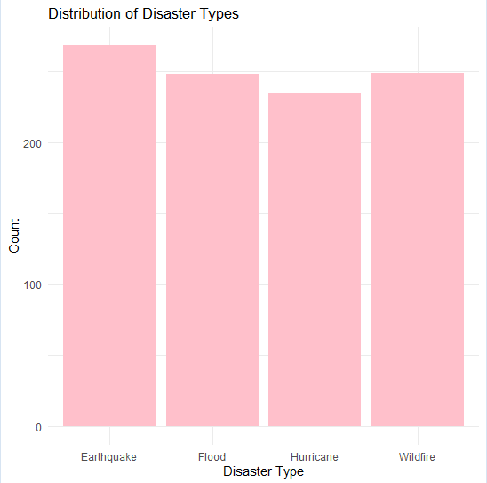
Distribution of Disaster types

**Analyze Magnitude Over Time

Show how the magnitude of disasters changes over time.

R `

ggplot(data_cleaned, aes(x = Date, y = Magnitude)) + geom_line(color = "red") + theme_minimal() + labs(title = "Magnitude of Disasters Over Time", x = "Date", y = "Magnitude")

`

**Output:

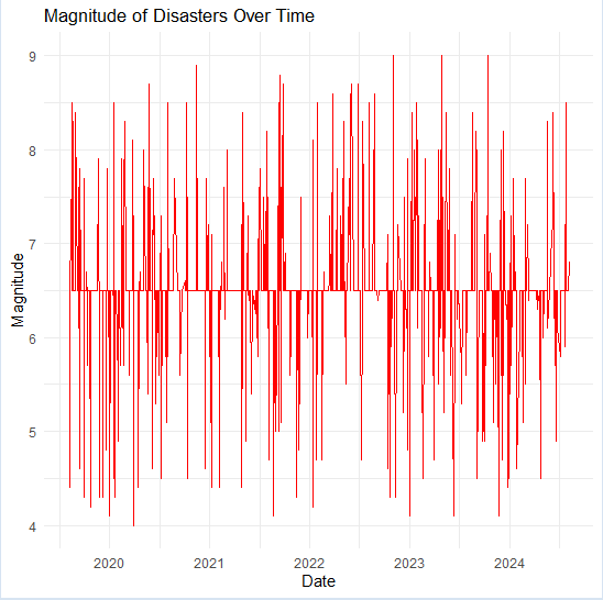
Plot Magnitude over time

**Location-Based Analysis

Display the geographical distribution of disasters.

R `

Location-Based Analysis

leaflet(data_cleaned) %>% addTiles() %>% addCircleMarkers(~Longitude, ~Latitude, color = ~Disaster_Type, popup = ~paste(Disaster_Type, "
", Date))

`

**Output:

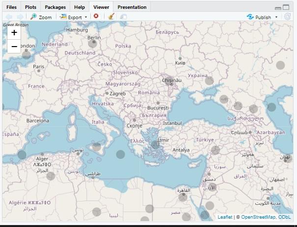
Natural Disaster Prediction in R

Step 4: Split the Data into Training and Testing Sets

• Used createDataPartition from caret to split the data into training (70%) and testing (30%) sets.
• Set a seed for reproducibility.
• Prepare separate datasets for training the model and evaluating its performance on unseen data. R `

Step 4: Split the Data into Training and Testing Sets

set.seed(42) # For reproducibility train_index <- createDataPartition(data_cleaned$Disaster_Type, p = 0.7, list = FALSE) train_data <- data_cleaned[train_index, ] test_data <- data_cleaned[-train_index, ]

`

Step 5: Train a Random Forest Model with Cross-Validation

• Defined a trainControl object for 10-fold cross-validation.
• Trained a Random Forest model using the training data with 10-fold cross-validation.
• Specified the independent variables (Latitude, Longitude, etc.) and the dependent variable (Disaster_Type).
• Used tuneLength = 5 to try 5 different values of mtry (number of variables randomly sampled as candidates at each split). R `

Step 5: Train a Random Forest Model with Cross-Validation and Reduced Complexity

control <- trainControl(method = "cv", number = 10)

Simplified model without additional parameters to prevent overfitting

model <- train( Disaster_Type ~ Latitude + Longitude + Magnitude + Depth + Wind_Speed + Rainfall + Temperature + Humidity + Historical_Frequency, data = train_data, method = "rf", trControl = control, tuneLength = 5 )

Check the Model Performance

print(model)

`

**Output:

Random Forest

702 samples
9 predictor
4 classes: 'Earthquake', 'Flood', 'Hurricane', 'Wildfire'

No pre-processing
Resampling: Cross-Validated (10 fold)
Summary of sample sizes: 630, 631, 633, 632, 632, 631, ...
Resampling results across tuning parameters:

mtry Accuracy Kappa
2 0.9899983 0.9866495
3 0.9928761 0.9904918
5 0.9928566 0.9904663
7 0.9928566 0.9904663
9 0.9928566 0.9904663

Accuracy was used to select the optimal model using the largest value.
The final value used for the model was mtry = 3.

**Step 6: Evaluate Model Performance

Now we will Print the Confusion Matrix to Evaluate Model Performance.

R `

Step 6: Predict on the Test Set

predictions <- predict(model, newdata = test_data)

#Evaluate the Model confusion_matrix <- confusionMatrix(predictions, test_data$Disaster_Type) cat("Confusion Matrix:\n") print(confusion_matrix)

Accuracy

cat("Accuracy:", round(confusion_matrix$overall['Accuracy'] * 100, 2), "%\n")

`

**Output:

Confusion Matrix:
Confusion Matrix and Statistics

        Reference  

Prediction Earthquake Flood Hurricane Wildfire
Earthquake 80 0 0 0
Flood 0 73 0 0
Hurricane 0 0 67 0
Wildfire 0 1 3 74

Overall Statistics

           Accuracy : 0.7866           
             95% CI : (0.966, 0.9963)  
No Information Rate : 0.2685           
P-Value [Acc > NIR] : < 2.2e-16        
                                       
              Kappa : 0.9821           
                                       

Mcnemar's Test P-Value : NA

Statistics by Class:

                 Class: Earthquake Class: Flood Class: Hurricane  

Sensitivity 1.0000 0.9865 0.9571
Specificity 1.0000 1.0000 1.0000
Pos Pred Value 1.0000 1.0000 1.0000
Neg Pred Value 1.0000 0.9956 0.9870
Prevalence 0.2685 0.2483 0.2349
Detection Rate 0.2685 0.2450 0.2248
Detection Prevalence 0.2685 0.2450 0.2248
Balanced Accuracy 1.0000 0.9932 0.9786
Class: Wildfire
Sensitivity 1.0000
Specificity 0.9821
Pos Pred Value 0.9487
Neg Pred Value 1.0000
Prevalence 0.2483
Detection Rate 0.2483
Detection Prevalence 0.2617
Balanced Accuracy 0.9911

Accuracy: 78.66 %

• Printed the trained model to check the optimal mtry value and the cross-validation accuracy.
• Made predictions on the test dataset.
• Generated a confusion matrix to evaluate the model’s performance on the test set.
• Calculated overall accuracy and Kappa statistics to assess model performance.

Step 7: Check for Overfitting with Out-of-Bag (OOB) Error

• Trained another Random Forest model, focusing on analyzing the OOB error rate.
• Printed the OOB error rate across different iterations.
• Determine if the model is overfitting by comparing the OOB error to the test set performance. R `

Step 7: Analyze Out-of-Bag (OOB) Error for Overfitting Check

rf_model_oob <- randomForest( Disaster_Type ~ Latitude + Longitude + Magnitude + Depth + Wind_Speed + Rainfall + Temperature + Humidity + Historical_Frequency, data = train_data, ntree = 200, mtry = 3, importance = TRUE, proximity = TRUE )

Print OOB error rate

cat("Out-of-Bag (OOB) Error Rate:\n") print(rf_model_oob$err.rate)

`

**Output:

Out-of-Bag (OOB) Error Rate:
OOB Earthquake Flood Hurricane Wildfire
[1,] 0.05200000 0.000000000 0.00000000 0.12698413 0.076923077
[2,] 0.04941176 0.026315789 0.01904762 0.06796117 0.087378641
[3,] 0.06156716 0.041095890 0.01515152 0.10156250 0.092307692
[4,] 0.05272109 0.025316456 0.02097902 0.08633094 0.081081081
[5,] 0.05537975 0.023668639 0.01910828 0.10273973 0.081250000
[6,] 0.03963415 0.022857143 0.01851852 0.06535948 0.054216867
[7,] 0.04154303 0.016759777 0.04191617 0.03750000 0.071428571
[8,] 0.05102041 0.027322404 0.04705882 0.05555556 0.076023392
[9,] 0.04310345 0.021505376 0.04624277 0.04268293 0.063583815
[10,] 0.04005722 0.021505376 0.04022989 0.04848485 0.051724138..................................................................................

Step 8: Predict values using model

Now we will Predict values using model.

R `

library(shiny)

Shiny UI

ui <- fluidPage( titlePanel("Interactive Disaster Data Analysis & Prediction"),

sidebarLayout( sidebarPanel( selectInput("disaster_type", "Choose Disaster Type:", choices = unique(data_cleaned$Disaster_Type)), dateRangeInput("date_range", "Select Date Range:", start = min(data_cleaned$Date), end = max(data_cleaned$Date)), numericInput("latitude", "Latitude:", value = 0), numericInput("longitude", "Longitude:", value = 0), numericInput("magnitude", "Magnitude:", value = 0), numericInput("depth", "Depth:", value = 0), numericInput("wind_speed", "Wind Speed:", value = 0), numericInput("rainfall", "Rainfall:", value = 0), numericInput("temperature", "Temperature:", value = 0), numericInput("humidity", "Humidity:", value = 0), numericInput("historical_freq", "Historical Frequency:", value = 0), actionButton("update", "Update"), actionButton("predict", "Predict Disaster Type") ),

mainPanel(
  tabsetPanel(
    tabPanel("Disaster Distribution", plotOutput("distPlot")),
    tabPanel("Magnitude Over Time", plotOutput("magnitudePlot")),
    tabPanel("Location Analysis", leafletOutput("mapPlot")),
    tabPanel("Prediction Result", textOutput("predictionResult"))
  )
)

) )

Shiny Server

server <- function(input, output, session) {

filtered_data <- reactive({ req(input$update) isolate({ data_cleaned %>% filter(Disaster_Type == input$disaster_type, Date >= input$date_range[1], Date <= input$date_range[2]) }) })

output$distPlot <- renderPlot({ ggplot(filtered_data(), aes(x = Disaster_Type)) + geom_bar(fill = "pink") + theme_minimal() + labs(title = "Distribution of Disaster Types", x = "Disaster Type", y = "Count") })

output$magnitudePlot <- renderPlot({ ggplot(filtered_data(), aes(x = Date, y = Magnitude)) + geom_line(color = "red") + theme_minimal() + labs(title = "Magnitude of Disasters Over Time", x = "Date", y = "Magnitude") })

output$mapPlot <- renderLeaflet({ leaflet(filtered_data()) %>% addTiles() %>% addCircleMarkers(~Longitude, ~Latitude, color = ~Disaster_Type, popup = ~paste(Disaster_Type, "
", Date)) })

observeEvent(input$predict, { new_data <- data.frame( Latitude = input$latitude, Longitude = input$longitude, Magnitude = input$magnitude, Depth = input$depth, Wind_Speed = input$wind_speed, Rainfall = input$rainfall, Temperature = input$temperature, Humidity = input$humidity, Historical_Frequency = input$historical_freq )

prediction <- predict(model, newdata = new_data)

output$predictionResult <- renderText({
  paste("Predicted Disaster Type:", prediction)
})

}) }

Run the Shiny App

shinyApp(ui = ui, server = server)

`

**Output:

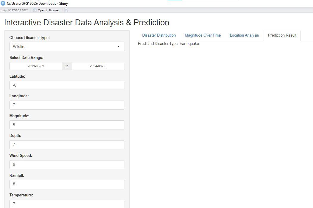
Natural Disaster Prediction in R

• **User Interface (UI):
  • The app's title is set with titlePanel("Interactive Disaster Data Analysis & Prediction").
• **Sidebar Layout:
  • selectInput() for choosing disaster types.
  • dateRangeInput() for selecting the date range.
  • numericInput() for entering numeric values related to disaster parameters (latitude, longitude, magnitude, etc.).
  • actionButton() to trigger data updates and predictions.
• **Main Panel:
  • Four tabs are created: "Disaster Distribution", "Magnitude Over Time", "Location Analysis", and "Prediction Result".
  • Each tab is designed to display a different output: plots, maps, or prediction results.
• **Server **Logic:
  • filtered_data() reacts to the "Update" button to filter data based on the selected disaster type and date range.
  • renderPlot() creates a bar plot showing the distribution of disaster types.
  • renderPlot() generates a line plot depicting disaster magnitude over time.
  • renderLeaflet() creates an interactive map to visualize disaster locations.
• **Prediction Logic:
  • observeEvent() listens for the "Predict" button click.
  • The user inputs are compiled into a data frame.
  • The trained Random Forest model predicts the disaster type based on these inputs.
  • The prediction is displayed as text in the "Prediction Result" tab.
• **Running the App:
  • The shinyApp() function combines the UI and server logic to run the Shiny application.

**Conclusion

Predicting natural disasters using data analysis in R helps us prepare better and respond more effectively. This article showed how to analyze disaster data and build a prediction model, helping us understand and manage natural disasters more efficiently.