OneWay ANOVA (original) (raw)
One-Way ANOVA
Last Updated : 23 Jan, 2026
Analysis of Variance (ANOVA) is a parametric statistical method used to determine whether there is a significant difference among the means of three or more groups by testing the null hypothesis that all group means are equal.
One Way Anova
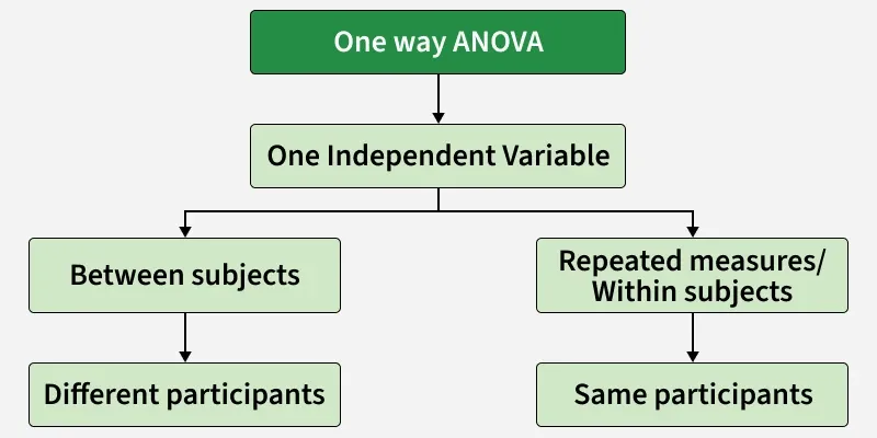
One-way ANOVA is the simplest form of ANOVA used when a single independent variable has three or more groups. It determines whether there are statistically significant differences among the group means by comparing within-group and between-group variation.
- One-way ANOVA analyzes the effect of a single factor on multiple independent groups.
- It is commonly used due to its simplicity and efficiency.
- The test indicates whether at least two group means differ, but does not identify which ones.
- It is mainly applied when three or more groups are compared.
- The relationship between one-way ANOVA and the t-test is given by F=t^{2}
Assumptions of ANOVA
- The dependent variable is approximately normally distributed within each group, especially important for small sample sizes.
- Observations are randomly selected and independent of one another.
- All groups have equal variances (homogeneity of variance).
- Each data point belongs to only one group with no overlap.
- For two-way ANOVA, the effects of independent variables are additive and there is no significant interaction between them.
When to Use One-Way ANOVA
A one-way Analysis of Variance (ANOVA) is used when you want to examine the effect of a single categorical independent variable on a quantitative dependent variable. The independent variable must consist of at least three distinct levels or groups.
One-way ANOVA determines whether the mean of the dependent variable differs significantly across the levels of the independent variable. Typical examples include:
- Website design version (Design A, Design B, Design C) as the independent variable and user engagement time as the dependent variable.
- Machine learning model type (Logistic Regression, SVM, Random Forest) as the independent variable and classification accuracy as the dependent variable.
- Social media usage level (low, medium, high) as the independent variable and average hours of sleep per night as the dependent variable.
The null hypothesis (H_{0}) states that all group means are equal, indicating no effect of the independent variable. The alternative hypothesis (H_{a}) states that at least one group mean differs significantly from the others.
How to Perform One-Way ANOVA
One-way ANOVA is a hypothesis test used to determine whether the means of three or more groups differ significantly based on a single factor. The test statistic used is the F-statistic which compares between-group variance to within-group variance.
Step 1: Define Hypotheses
- *Null hypothesis(H_{0}*): All group population means are equal
\mu_1 = \mu_2 = \mu_3 = \dots = \mu_k
- **Alternative hypothesis (H_{a}): At least one group mean differs.
This step clarifies what you are testing and what outcome would lead you to reject the null.
Step 2: Compute Degrees of Freedom
Degrees of freedom (df) help determine the critical F-value from statistical tables.
Between groups: df_{\text{between}} = k - 1
Within groups: df_{within} = n - k
df_{total} = df_{between} + df_{within}
where
- k: number of groups
- n: total number of observations
Step 3: Understand the F-Statistic
The F-statistic is the ratio of variability between groups to variability within groups:
F = \frac{\text{Variance between groups}}{\text{Variance within groups}}
A larger F-value indicates that group means differ more than expected by chance.
Step 4: Calculate Group Means and Grand Mean
Compute the mean of each group. Then calculate the grand mean across all observations:
\mu_{grand} = \frac{\sum G}{n}
where
- {\sum G} is the sum of all observations
- {n} is the total sample size Python `
import numpy as np
team_A = [50, 47, 52, 46, 51, 48, 49, 47, 50] team_B = [40, 42, 38, 41, 39, 40, 41, 39, 40] team_C = [55, 54, 57, 53, 56, 55, 55, 54, 57]
data = [team_A, team_B, team_C]
group_means = [np.mean(team) for team in data] overall_mean = np.mean([x for team in data for x in team])
print("Group Means:", dict(zip(['Team A','Team B','Team C'], group_means))) print("Overall Mean:", round(overall_mean, 2))
`
**Output:
Group Means: {'Team A': np.float64(48.888888888888886), 'Team B': np.float64(40.0), 'Team C': np.float64(55.111111111111114)}
Overall Mean: 48.0
Step 5: Compute Sum of Squares
Measure variability using sum of squares (SS)
**Total Sum of Squares:
SS_{total} = \sum (x_i - \mu_{grand})^2
**Within-Group Sum of Squares:
SS_{within} = \sum (x_i - \mu_i)^2
**Between-Group Sum of Squares:
SS_{between} = SS_{total} - SS_{within}
This separates variability due to group differences from random error.
Python `
SS_between = sum([len(team)*(np.mean(team)-overall_mean)**2 for team in data]) SS_within = sum([sum((x-np.mean(team))**2 for x in team) for team in data])
`
Step 6: Compute Mean Squares
Convert sums of squares into mean squares by dividing by their respective degrees of freedom
MS_{between} = \frac{SS_{between}}{df_{between}}
MS_{within} = \frac{SS_{within}}{df_{within}}
Python `
k = len(data) n = sum(len(team) for team in data)
df_between = k - 1 df_within = n - k
MS_between = SS_between / df_between MS_within = SS_within / df_within
`
Step 7: Calculate the F-Statistic
F_{calc} = \frac{MS_{between}}{MS_{within}}
This is the test statistic used to compare against the critical F-value.
Python `
F_stat = MS_between / MS_within from scipy import stats
p_value = 1 - stats.f.cdf(F_stat, df_between, df_within) print(f"F-statistic: {F_stat:.4f}")
`
**Output:
F-statistic: 208.4164
Step 8: Test Assumptions
- **Normality: Each group should be normally distributed.
- **Equal variance: Variances across groups should be similar. Python `
for i, team in enumerate(data, start=1): stat, p = stats.shapiro(team) print(f"Team {chr(64+i)} p-value: {p:.4f}")
stat, p = stats.levene(*data) print(f"Levene's Test p-value: {p:.4f}")
`
**Output:
Team A p-value: 0.7796
Team B p-value: 0.8299
Team C p-value: 0.4944
Levene's Test p-value: 0.1541
Step 9: Making the Statistical Decision
After computing the F-statistic, decide whether to reject or fail to reject H_{0}
**1. Using the F-Table
Compare the calculated F-value (F_{calc}) with the critical F-value from the F-distribution table (F_{table}) at the chosen significance level (\alpha):
- if F_{calc} < F_{table}: Do not reject H_{0} all group means are equal
- if F_{calc} > F_{table} : Reject H_{0} at least one group mean is significantly different
**2. Using the p-value
Compare p-value with significance level \alpha:
Python `
alpha = 0.05 if p_value < alpha: print("Reject H0: At least one team mean is significantly different") else: print("Fail to reject H0: No significant difference between team means")
`
**Output:
Reject H0: At least one team mean is significantly different
You can download full code from here
Advantages
- Can test multiple groups simultaneously, unlike t-tests which are limited to two groups.
- Reduces the Type I error that occurs when performing multiple t-tests.
- Easy to implement and interpret with statistical software.
- Provides a quantitative measure (F-statistic) to evaluate group differences.
Limitations
- Assumes normality, homogeneity of variances and independence of observations.
- Only identifies that a difference exists, not which specific groups differ (requires post-hoc tests).
- Sensitive to outliers, which can distort results.
- Cannot handle more than one independent variable; for that, two-way ANOVA is needed.