Particle Swarm Optimization (PSO) (original) (raw)

Last Updated : 10 Feb, 2026

Optimisation aims to find the best solution from a set of feasible options under given constraints. In many machine learning and engineering problems, the search space is complex, non-linear and multimodal, where traditional gradient-based methods may be ineffective. This makes population-based optimization techniques more suitable.

PSo100

Particle Swarm Optimization

Particle Swarm Optimization (PSO) is a stochastic population based optimization technique inspired by swarm intelligence in nature. It is designed to solve complex optimization problems where the search space is large, non-linear or unknown, where traditional deterministic methods are ineffective.

Each particle represents a potential solution and moves through the search space
Movement is guided by both individual experience and collective swarm knowledge
The algorithm iteratively improves solutions using a fitness function
Simple to implement with fast convergence and few control parameters

How Particle Swarm Optimization (PSO) Works

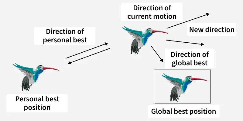
Particle Swarm Optimization (PSO) is an iterative, population based optimization algorithm. It works by moving a group of particles (candidate solutions) through the search space using simple mathematical rules based on personal and collective experience.

Each particle in PSO has

**Position (x): current solution
**Velocity (v): direction and speed of movement
**Fitness value: quality of the solution

Each particle stores:

**pBest: best position found by itself
**gBest: best position found by the entire swarm

frame_3315

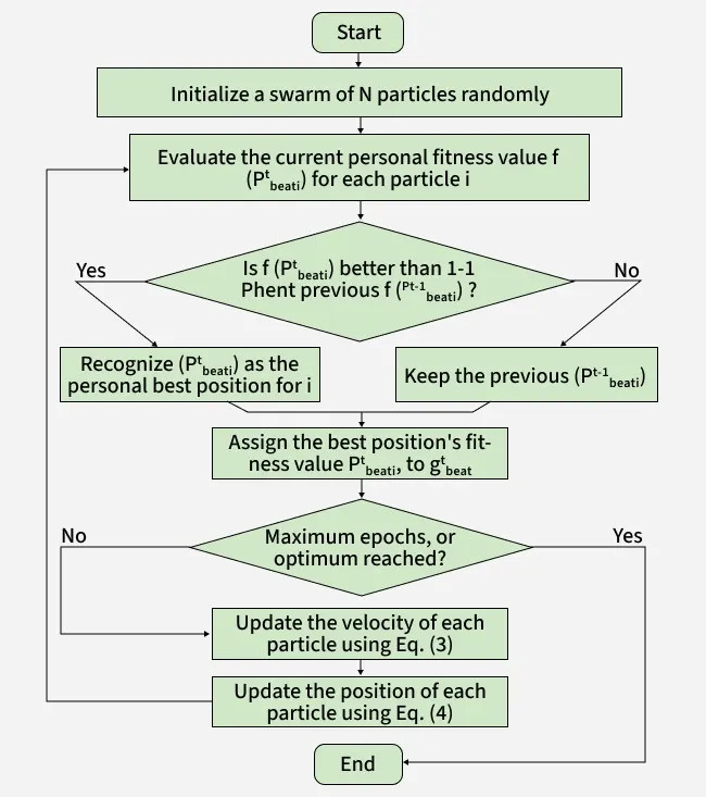
PSO Workflow

Step 1: Initialization

Randomly initialize N particles within the search space [minx,maxx]
Assign a random velocity to each particle
Evaluate the fitness value of each particle

pBest = current position
gBest = best pBest among all particles

Step 2: Velocity Update

At each iteration the velocity of a particle is updated using:

v_{i}^{t+1} = w \cdot v_{i}^{t} + c_{1} \cdot r_{1} \cdot (pBest_{i} - x_{i}^{t}) + c_{2} \cdot r_{2} \cdot (gBest - x_{i}^{t})

where

w: inertia weight (controls exploration)
{c_1}: cognitive coefficient (self-learning)
c_2: social coefficient (swarm learning)
{r_1},{r_2}: random values in [0,1]

Step 3: Position Update

After updating velocity the position is updated as:

x_{i}^{t+1} = x_{i}^{t} + v_{i}^{t+1}

If the new position goes outside [minx,maxx] clip it to the boundary.

Step 4: Update Best Positions

If current fitness is better than pBest, update pBest
If current fitness is better than gBest, update gBest

Step 5: Convergence

Repeat Steps 2–4 for a fixed number of iterations or until convergence
The swarm gradually moves toward the optimal solution

Step By Step Implementation

Here in this code we implements Particle Swarm Optimization (PSO) to find the global minimum of the Ackley function by iteratively updating a swarm of particles based on their personal best and the global best positions.

It simulates collective behavior to efficiently search the solution space and converge to an optimal solution.

Step 1: Import Required Libraries

Import numpy for numerical computations and vector operations
Import math for mathematical constants and functions
Import matplotlib.pyplot for possible visualization Python `

import numpy as np import math import matplotlib.pyplot as plt

Step 2: Define the Cost (Objective) Function

The Ackley function is a common benchmark function for optimization algorithms
It is multimodal, non-convex and difficult for gradient-based methods
PSO aims to minimize this function Python `

def cost_function(x): a = 20 b = 0.2 c = 2 * math.pi d = len(x)

term1 = -a * np.exp(-b * np.sqrt(np.sum(x**2) / d))
term2 = -np.exp(np.sum(np.cos(c * x)) / d)

return term1 + term2 + a + math.e

Step 3: Define PSO Hyperparameters

**DIMENSIONS: specifies the search space dimensionality
**POPULATION: represents the number of particles
**MAX_ITER: controls the number of optimization iterations
**MIN_BOUND and MAX_BOUND: define the search space limits
**w, c1 and c2: are inertia, cognitive and social coefficients Python `

DIMENSIONS = 2 POPULATION = 30 MAX_ITER = 100

MIN_BOUND = -5 MAX_BOUND = 5

w = 0.7 c1 = 1.5 c2 = 1.5 V_MAX = 0.5

Step 4: Define the Particle Class

Each particle represents a candidate solution
Particles have position, velocity and personal best
Fitness is calculated using the cost function
Personal best is updated whenever a better solution is found Python `

class Particle: def init(self): self.position = np.random.uniform(MIN_BOUND, MAX_BOUND, DIMENSIONS) self.velocity = np.random.uniform(-V_MAX, V_MAX, DIMENSIONS) self.best_position = self.position.copy() self.best_fitness = cost_function(self.position) self.fitness = self.best_fitness

Step 5: Initialize the Swarm and Global Best

A swarm of particles is created
The global best solution is selected from all personal bests
This global best guides the swarm during optimization Python `

def particle_swarm_optimization(): swarm = [Particle() for _ in range(POPULATION)]

gbest_position = swarm[0].best_position.copy()
gbest_fitness = swarm[0].best_fitness

for particle in swarm:
    if particle.best_fitness < gbest_fitness:
        gbest_fitness = particle.best_fitness
        gbest_position = particle.best_position.copy()

Step 6: Update Velocity and Position of Particles

Velocity update includes inertia, cognitive and social components
Random factors introduce stochastic behavior
Velocity and position are clipped to avoid divergence
This step enables exploration and exploitation Python `

for iteration in range(MAX_ITER): for particle in swarm: r1 = np.random.rand(DIMENSIONS) r2 = np.random.rand(DIMENSIONS) particle.velocity = ( w * particle.velocity + c1 * r1 * (particle.best_position - particle.position) + c2 * r2 * (gbest_position - particle.position) ) particle.velocity = np.clip(particle.velocity, -V_MAX, V_MAX) particle.position = particle.position + particle.velocity particle.position = np.clip(particle.position, MIN_BOUND, MAX_BOUND)

Step 7: Update Personal Best and Global Best

Fitness is recalculated after position update
Personal best is updated if a better fitness is achieved

Global best is updated if any particle outperforms the current best Python `

      particle.fitness = cost_function(particle.position)

      if particle.fitness < particle.best_fitness:
          particle.best_fitness = particle.fitness
          particle.best_position = particle.position.copy()

      if particle.fitness < gbest_fitness:
          gbest_fitness = particle.fitness
          gbest_position = particle.position.copy()

  print(f"Iteration {iteration+1}/{MAX_ITER}, Best Fitness = {gbest_fitness:.6f}")

return gbest_position, gbest_fitness

Step 8: Execute the PSO Algorithm

The PSO function is executed from the main block
Final optimal position and fitness value are printed
The result approximates the global minimum of the Ackley function Python `

if name == "main": best_position, best_fitness = particle_swarm_optimization()

print("\nOptimal Solution Found:")
print("Best Position:", best_position)
print("Best Fitness:", best_fitness)

**Output:

PSO8

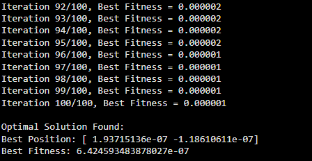
Output

You can download full code from here

Difference between Particle Swarm Optimization (PSO) and Genetic Algorithm (GA)

Here we compare Particle Swarm Optimization (PSO) and Genetic Algorithm(GA):

Parameter	PSO	Genetic Algorithm (GA)
Inspiration	Based on social behavior of birds or fish	Based on natural evolution and genetics
Search Strategy	Particles move continuously through the search space	Uses randomized population evolution
Population Update	No creation or deletion particles only change position	New individuals are created using crossover and mutation
Operators Used	Velocity and position updates	Selection, crossover and mutation
Variable Handling	Best suited for continuous optimization	Handles both continuous and discrete variables
Complexity and Speed	Simple structure with faster convergence	More complex and generally slower

Application

1. Health Care Applications

**Intelligent Diagnosis: Optimizes models for faster and accurate disease detection.
**Medical Robots: Guides robots for precise surgical or therapeutic tasks.

2. Environmental Applications

**Wild Vegetation Monitoring: Tracks forest and vegetation growth efficiently.
**Agriculture Monitoring: Optimizes crop management and environmental monitoring.
**Flood Control and Routing: Predicts floods and finds optimal evacuation or routing paths.

3. Industrial Applications

**WSN Deployment: Optimizes sensor placement in Wireless Sensor Networks.
**Product Defection Prediction: Predicts defects to improve product quality.
**Microgrid Design and Operation: Optimizes design and operation for stability.

4 Smart City Applications

**Smart City Planning: Optimizes urban energy, traffic and resources.
**Smart Home Automation: Efficiently controls and schedules home appliances.
**Appliance Scheduling: Reduces energy consumption via optimal use.

Advantages

Simple to implement with fewer control parameters.
Fast convergence compared to many traditional algorithms.
Does not require gradient information.
Effective for non-linear and multimodal problems.
Easily used with other optimization techniques.

Limitations

May converge early to local optima.
Weak local search capability in later iterations.
Performance depends on proper parameter tuning.
Computational cost increases with swarm size.
Less effective for discrete optimization problems.