Predicting Stock Price Direction using Support Vector Machines (original) (raw)

Last Updated : 23 Jul, 2025

Predicting stock price direction is a key goal for traders and analysts. Support Vector Machines (SVM) is a machine learning algorithm that can help classify whether a stock's price will rise or fall. In this article, we'll demonstrate how to apply SVM to predict stock price movements using historical data, covering data preparation, model training, and evaluation.

Step-by-Step Implementation

Step 1: Import the libraries

Here we will import pandas, scikit learn and matplotlib.

Python `

Machine learning

from sklearn.svm import SVC from sklearn.metrics import accuracy_score

For data manipulation

import pandas as pd import numpy as np

To plot

import matplotlib.pyplot as plt

To ignore warnings

import warnings warnings.filterwarnings("ignore")

`

Step 2: Read Stock data

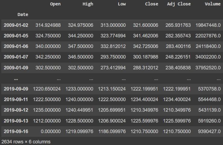
We will Read the Stock Data Downloaded From Yahoo Finance Website. You can download dataset from **here****.**

Python `

Read the csv file using read_csv

method of pandas

df = pd.read_csv('RELIANCE.csv') df

`

**Output:

dataset

Step 3: Data Preparation

The data needed to be processed before use such that the date column should act as an index to do that and will drop date column.

Python `

Changes The Date column as index columns

df.index = pd.to_datetime(df['Date']) df

drop The original date column

df = df.drop(['Date'], axis='columns') df

`

**Output:

Data Preparation

Step 4: Define the explanatory variables

Explanatory or independent variables are used to predict the value response variable. The X is a dataset that holds the variables which are used for prediction. The X consists of variables such as 'Open - Close' and 'High - Low'. These can be understood as indicators based on which the algorithm will predict tomorrow's trend. Feel free to add more indicators and see the performance.

Python `

Create predictor variables

df['Open-Close'] = df.Open - df.Close df['High-Low'] = df.High - df.Low

Store all predictor variables in a variable X

X = df[['Open-Close', 'High-Low']] X.head()

`

**Output:

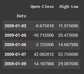
Explanatory variables

Step 5: Define the target variable

The target variable is the outcome which the machine learning model will predict based on the explanatory variables. If tomorrow's price is greater than today's price then we will buy the particular Stock else we will have no position in the. We will store +1 for a buy signal and 0 for a no position in y. We will use where() function from NumPy to do this.

Python `

Target variables

y = np.where(df['Close'].shift(-1) > df['Close'], 1, 0) y

`

**Output:

array([1, 1, 0, ..., 1, 0, 0])

Step 6: Split the data into train and test

We will split data into training and test data sets. This is done so that we can evaluate the effectiveness of the model in the test dataset. We will split 80% data for training and 20% for testing.

Python `

split_percentage = 0.8 split = int(split_percentage*len(df))

Train data set

X_train = X[:split] y_train = y[:split]

Test data set

X_test = X[split:] y_test = y[split:]

`

Step 7: Support Vector Classifier (SVC)

We will use Support Vector Machines by SVC() function from sklearn.svm.SVC library to create our classifier model using the fit() method on the training data set.

Python `

Support vector classifier

cls = SVC().fit(X_train, y_train)

`

Step 8: Classifier accuracy

This code calculates and prints the accuracy of your model on both the training and testing data which were split 80/20 to check for overfitting.

Python `

print("The data was split into training and testing sets using an 80/20 split.")

Calculate training accuracy

train_accuracy = accuracy_score(y_train, cls.predict(X_train))

Calculate testing accuracy

test_accuracy = accuracy_score(y_test, cls.predict(X_test))

print(f"Training Accuracy: {train_accuracy}") print(f"Testing Accuracy: {test_accuracy}")

`

**Output:

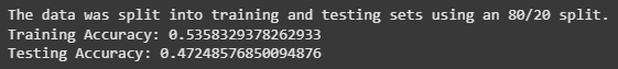
Training and testing accuracy

Step 9: Different Kernels

This code trains and tests SVC models with different kernels like linear, polynomial, RBF and sigmoid to see how the kernel affects prediction accuracy on the test data. It then prints the accuracy for each kernel.

Python `

from sklearn.metrics import accuracy_score

Linear kernel

cls_linear = SVC(kernel='linear').fit(X_train, y_train) y_pred_linear = cls_linear.predict(X_test) accuracy_linear = accuracy_score(y_test, y_pred_linear) print(f"Accuracy with Linear Kernel: {accuracy_linear}")

Polynomial kernel

cls_poly = SVC(kernel='poly', degree=3).fit(X_train, y_train) y_pred_poly = cls_poly.predict(X_test) accuracy_poly = accuracy_score(y_test, y_pred_poly) print(f"Accuracy with Polynomial Kernel (degree=3): {accuracy_poly}")

RBF kernel (default)

cls_rbf = SVC(kernel='rbf').fit(X_train, y_train) y_pred_rbf = cls_rbf.predict(X_test) accuracy_rbf = accuracy_score(y_test, y_pred_rbf) print(f"Accuracy with RBF Kernel: {accuracy_rbf}")

Sigmoid kernel

cls_sigmoid = SVC(kernel='sigmoid').fit(X_train, y_train) y_pred_sigmoid = cls_sigmoid.predict(X_test) accuracy_sigmoid = accuracy_score(y_test, y_pred_sigmoid) print(f"Accuracy with Sigmoid Kernel: {accuracy_sigmoid}")

`

**Output:

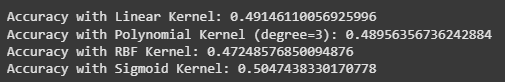
Accuracy with different Kernels

Step 10: Strategy implementation

We will predict the signal (buy or sell) using the cls.predict() function.

Python `

df['Predicted_Signal'] = cls.predict(X)

`

Calculate Daily returns

Python `

Calculate daily returns

df['Return'] = df.Close.pct_change()

`

Calculate Strategy Returns

Python `

Calculate strategy returns

df['Strategy_Return'] = df.Return *df.Predicted_Signal.shift(1)

`

Calculate Cumulative Returns

Python `

Calculate Cumulutive returns

df['Cum_Ret'] = df['Return'].cumsum() df

`

**Output :

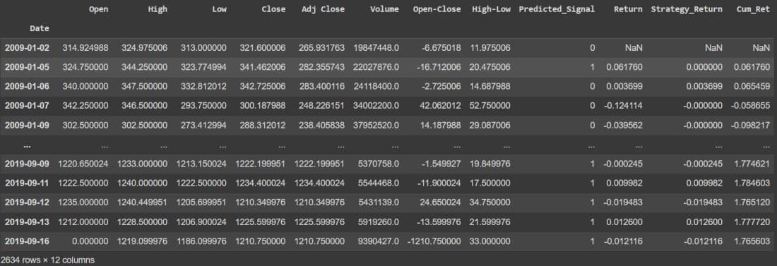
Calculate Cumulative Returns

Calculate Strategy Cumulative Returns

Python `

Plot Strategy Cumulative returns

df['Cum_Strategy'] = df['Strategy_Return'].cumsum() df

`

**Output

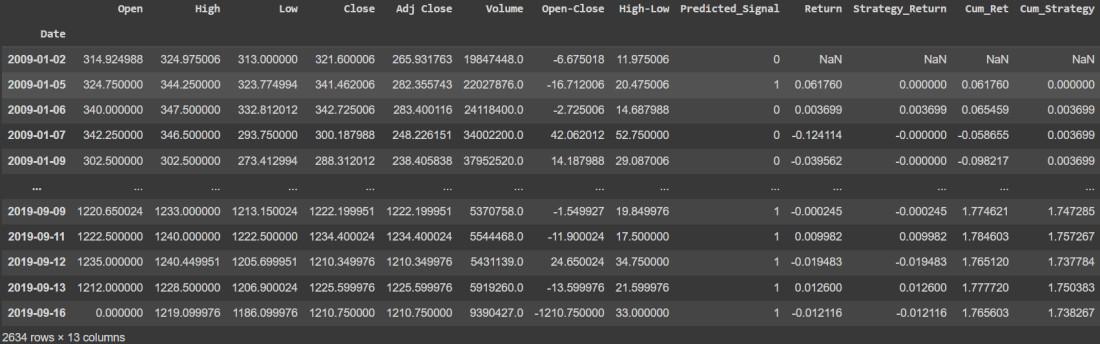
Calculate Strategy Cumulative Returns

Step 11: Visualizing Strategy Returns vs Original Returns

Python `

import matplotlib.pyplot as plt %matplotlib inline

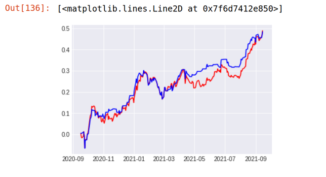
plt.plot(Df['Cum_Ret'],color='red') plt.plot(Df['Cum_Strategy'],color='blue')

`

**Output:

Plot Strategy Returns vs Original Returns

As You Can See Our Strategy Seem to be Totally Outperforming the Performance of The Reliance Stock. Our Strategy (Blue Line) Provided the return of 18.87 % in the last 1 year whereas the stock of Reliance Industries (Red Line) Provides the Return of just 5.97% in the last 1 year. We can further fine tune our model for better accuracy.

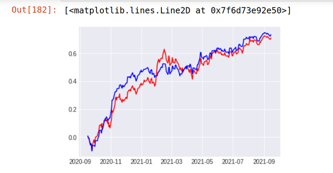
Step 12: Let's see our model result on different stocks

**1. TCS

Stock Return Over Last 1 year - 48% Strategy result - 48.9 %

**2. ICICI BANK

Stock Return Over Last 1 year - 48% Strategy result - 48.9 %

**Get the complete notebook link from here:

**Notebook link : **click here.