Pruning Decision Trees (original) (raw)

Last Updated : 2 Feb, 2026

Decision trees, when allowed to grow freely, tend to learn noise and very specific patterns from the training data, leading to overfitting. Pruning addresses this issue by simplifying the tree structure, improving generalization to unseen data, enhancing interpretability and reducing computational cost, while maintaining or even improving overall model accuracy.

• Reduces overfitting by eliminating noise-driven splits
• Improves generalization on unseen data
• Simplifies the decision tree structure
• Enhances interpretability of decision rules
• Improves training and inference efficiency

Decision Tree Pruning is a model optimization technique used to control the growth of decision tree models by removing unnecessary branches and nodes that do not contribute significantly to predictive performance.

Types of Decision Tree Pruning

Decision tree pruning techniques are broadly classified into two categories:

1. Pre-Pruning (Early Stopping)

Pre-pruning is also known as early stopping, is a pruning strategy in which the growth of the decision tree is restricted during the training phase itself. Instead of allowing the tree to grow fully and then trimming it later, pre-pruning prevents certain splits from being created if they do not satisfy predefined constraints.

• Controls tree complexity during training
• Prevents unnecessary splits early in the learning process
• Produces compact and shallow trees
• Reduces training time and memory usage

Working

• The decision tree starts growing from the root node using training data
• At each node, the algorithm checks whether a split satisfies predefined conditions
• If the split improves impurity reduction and meets constraints, the node is split
• If the split does not meet conditions, the node is converted into a leaf
• Constraints such as maximum depth or minimum samples control further growth
• Tree growth stops early before it becomes overly complex
• The final tree remains shallow and simple

Common Pre-Pruning Techniques

**1. Maximum Depth

• Limits the depth of the tree
• Prevents long and complex decision paths

**2. Minimum Samples per Split

• Requires a minimum number of samples to split a node
• Avoids unreliable splits based on small datasets

**3. Minimum Samples per Leaf

• Ensures each leaf node contains enough samples
• Reduces sensitivity to noise and outliers

**4. Maximum Features

• Limits the number of features considered at each split
• Introduces randomness and reduces overfitting

2. Post-Pruning (Pruning After Full Growth)

Post-pruning is a pruning strategy in which the decision tree is allowed to grow to its full depth first, after which unnecessary or weak branches are removed. Unlike pre-pruning, this approach does not restrict the tree during training. Instead, it analyzes the fully grown tree and evaluates whether certain subtrees contribute meaningfully to predictive performance.

• Applied after the tree is fully grown
• Uses validation or test performance for pruning decisions
• Produces well-balanced trees with better generalization
• Typically results in higher predictive stability

Working

• The decision tree is first grown completely using the training dataset
• All possible splits are created without restricting tree depth
• The fully grown tree is then evaluated using validation or test data
• Branches that do not improve prediction accuracy are identified
• Weak or unnecessary subtrees are removed from the tree
• Removed branches are replaced with leaf nodes
• The final tree is simpler while maintaining strong generalization performance

Common Post-Pruning Techniques

**1. Cost-Complexity Pruning (CCP)

• Introduces a penalty for tree complexity
• Uses a pruning parameter (α) to balance accuracy and size

**2. Reduced Error Pruning

• Removes branches that do not improve validation accuracy

**3. Minimum Impurity Decrease

• Prunes nodes with very small impurity reduction

**4. Minimum Leaf Size

• Removes leaf nodes with insufficient samples

Implementation

Let's see the implementation using the Breast cancer dataset from scikit-learn.

Step 1: Import Libraries and Load Dataset

We need to import the required libraries and load the dataset from scikit-learn library.

Python `

from sklearn.datasets import load_breast_cancer from sklearn.model_selection import train_test_split from sklearn.tree import DecisionTreeClassifier, plot_tree import matplotlib.pyplot as plt

`

Step 2: Split the Dataset

• Loads features and labels
• Splits data into training and testing sets
• Ensures reproducibility using a fixed random state Python `

X, y = load_breast_cancer(return_X_y=True)

X_train, X_test, y_train, y_test = train_test_split( X, y, train_size=0.2, random_state=42 )

`

Step 3: Train the Original (Unpruned) Decision Tree

• Uses Gini impurity to measure split quality
• Trains a fully grown decision tree Python `

model = DecisionTreeClassifier(criterion="gini") model.fit(X_train, y_train)

`

**Output:

Model Training

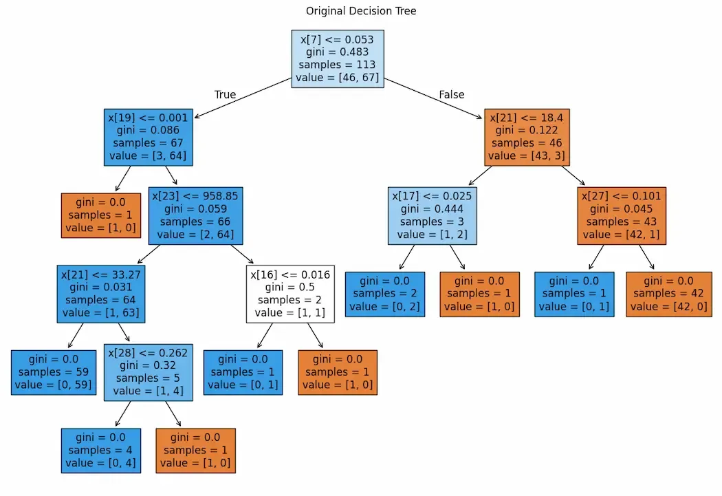
Step 4: Visualize the Original Decision Tree

• Large figure size improves node spacing
• Reduced font size avoids overlap
• Filled nodes reflect class purity Python `

plt.figure(figsize=(20, 12)) plot_tree( model, filled=True, fontsize=11 ) plt.title("Original Decision Tree", fontsize=18) plt.show()

`

**Output:

Output

Step 5: Model Accuracy Before Pruning

Here we evaluates baseline model performance

Python `

accuracy_before_pruning = model.score(X_test, y_test) print("Accuracy before pruning:", accuracy_before_pruning)

`

**Output:

Accuracy before pruning: 0.8947368421052632

Step 6: Hyperparameter Grid and GridSearchCV

• Defines constraints to limit tree complexity
• Uses cross-validation to find optimal settings Python `

from sklearn.model_selection import GridSearchCV

parameters = { 'criterion': ['gini', 'entropy', 'log_loss'], 'splitter': ['best', 'random'], 'max_depth': [1, 2, 3, 4, 5], 'max_features': ['sqrt', 'log2'] }

dt = DecisionTreeClassifier() cv = GridSearchCV(dt, param_grid=parameters, cv=5) cv.fit(X_train, y_train)

`

**Output:

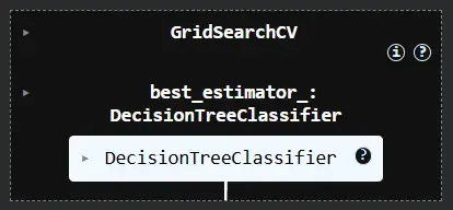
GridSearchCV

Step 7: Evaluate the Pre-Pruned Model

• Displays performance after pre-pruning
• Shows optimal hyperparameter values Python `

print("Best Accuracy:", cv.score(X_test, y_test)) print("Best Parameters:", cv.best_params_)

`

**Output:

Best Accuracy: 0.9276315789473685
Best Parameters: {'criterion': 'entropy', 'max_depth': 4, 'max_features': 'log2', 'splitter': 'best'}

Step 8: Compute Pruning Path

• Computes pruning strength values
• Higher alpha values lead to simpler trees Python `

path = model.cost_complexity_pruning_path(X_train, y_train) ccp_alphas = path.ccp_alphas

`

Step 9: Train Pruned Models

• Trains trees with varying levels of pruning
• Creates models with different complexities Python `

pruned_models = []

for alpha in ccp_alphas: pruned_model = DecisionTreeClassifier( criterion="gini", ccp_alpha=alpha ) pruned_model.fit(X_train, y_train) pruned_models.append(pruned_model)

`

Step 10: Select the Best Pruned Model

• Evaluates each pruned model
• Selects the best-performing one Python `

best_accuracy = 0 best_pruned_model = None

for m in pruned_models: acc = m.score(X_test, y_test) if acc > best_accuracy: best_accuracy = acc best_pruned_model = m

print("Accuracy after pruning:", best_accuracy)

`

**Output:

Accuracy after pruning: 0.9166666666666666

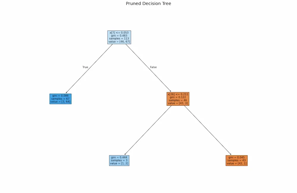
Step 11: Visualize the Pruned Decision Tree

• Increased spacing improves readability
• Shows a simplified and interpretable tree Python `

plt.figure(figsize=(22, 14)) plot_tree( best_pruned_model, filled=True, fontsize=11 ) plt.title("Pruned Decision Tree", fontsize=18) plt.show()

`

**Output:

Output

Advantages

• **Prevents Overfitting: Pruning removes branches that capture noise and overly specific patterns from training data, reducing memorization and improving real-world performance.
• **Improves Generalization: By simplifying the tree structure, pruning helps the model learn meaningful patterns that perform better on unseen data.
• **Reduces Model Complexity: Pruning decreases the number of nodes and branches, resulting in a compact model with lower computational and memory requirements.
• **Enhances Interpretability: A pruned decision tree is easier to understand, as it contains fewer decision paths and clearer logical rules.
• **Speeds Up Prediction: With fewer nodes to evaluate, pruned trees produce faster predictions during inference.