Regression using LightGBM (original) (raw)

Last Updated : 5 Sep, 2025

LightGBM (Light Gradient Boosting Machine) is an open-source gradient boosting framework designed for efficient and scalable machine learning. It works for both structured and unstructured data and is optimized for speed and memory usage.

• Handles large datasets with millions of rows and columns
• Supports parallel and distributed computing
• Uses histogram-based techniques and leaf-wise tree growth for efficiency
• Provides options like Exclusive Feature Bundling (EFB) and Gradient-based One-Side Sampling (GOSS) for faster computation and reduced memory usage

Working of LightGBM

LightGBM builds trees leaf-wise (splitting the leaf with the highest gain) rather than level-wise, which can improve accuracy but may overfit smaller datasets.

• Uses histograms to bucket continuous values and reduce computations
• Leaf-wise tree growth selects splits with maximum gain
• Exclusive Feature Bundling reduces feature dimensionality
• GOSS prioritizes instances with larger gradients to improve learning efficiency

Implementation of LightGBM

We will implement regression using LightGBM, covering library installation, data loading, preprocessing, training and evaluation.

1. Installing Libraries

We will install LightGBM for regression tasks.

• pip install lightgbm==3.3.5 installs a specific version compatible with our notebook

!pip install lightgbm==3.3.5

2. Importing Libraries and Dataset

We will import the necessary Python libraries such as pandas, numpy, seaborn, matplotlib, sklearn and load the dataset.

The used dataset can be downloaded from here.

Python `

import pandas as pd import numpy as np import seaborn as sb import matplotlib.pyplot as plt import lightgbm as lgb

from sklearn.preprocessing import StandardScaler from sklearn.model_selection import train_test_split from sklearn.metrics import mean_squared_error as mse from lightgbm import LGBMRegressor

import warnings warnings.filterwarnings('ignore')

df = pd.read_csv('medical_cost.csv')

`

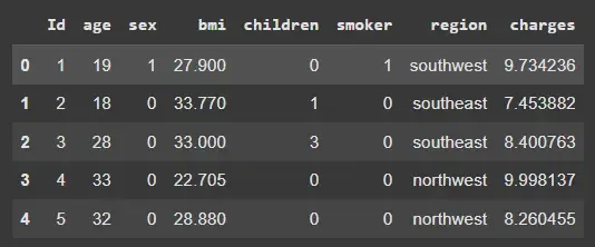
2.1. Previewing the Dataset

We will check the first few rows to understand the data structure.

• **df.head(): Displays the first five rows for a quick preview Python `

df.head()

`

**Output:

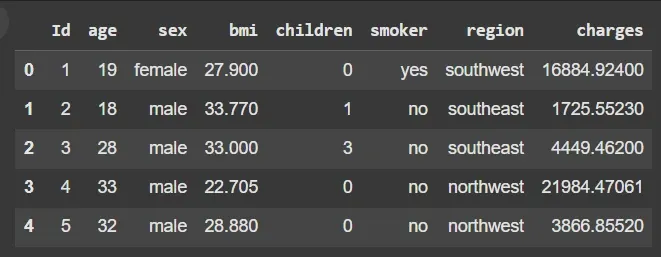
Dataset

2.2. Dataset Shape

We will check the dimensions of the dataset.

• **df.shape: Returns the number of rows and columns Python `

df.shape

`

**Output:

(1338, 8)

2.3. Dataset Information

We will check the data types and null values.

• **df.info(): Displays column data types and counts of non-null values Python `

df.info()

`

**Output:

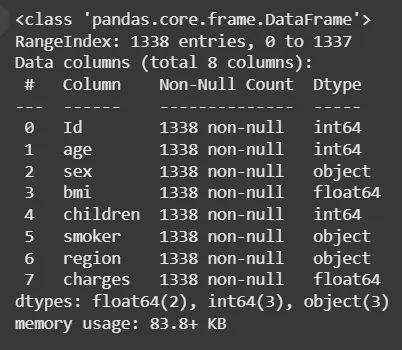
Information of Dataset

2.4. Descriptive Statistics

We will compute statistical summaries of numeric features.

• **df.describe(): Shows count, mean, std, min, max and percentiles Python `

df.describe()

`

**Output:

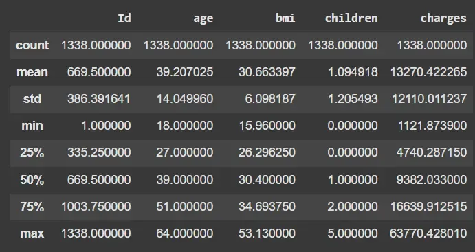
Description

3. Exploratory Data Analysis (EDA)

We will analyze patterns, distributions and relationships among features.

3.1: Mean Charges by Categorical Columns

We will calculate average charges for each category in categorical features.

• **groupby(col).mean(): Computes mean charges per category Python `

categorical_cols = ['sex', 'children', 'smoker', 'region']

for col in categorical_cols: grouped_data = df[[col, 'charges']].groupby(col).mean() print(f"Mean charges by {col}:") print(grouped_data) print()

`

**Output:

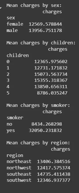
Mean Charges

3.2. Visualizing Categorical Distributions

We will plot count distributions for categorical columns.

• **countplot(): Displays counts for each category
• Helps identify balance or skew in categorical features Python `

plt.subplots(figsize=(15, 15)) for i, col in enumerate(categorical_cols): plt.subplot(3, 2, i + 1) sb.countplot(data=df, x=col) plt.tight_layout() plt.show()

`

**Output:

3.3. Visualizing Numerical Distributions

We will plot histograms of numerical features to check skewness and spread.

• **histplot(): Plots distribution with optional KDE for density Python `

numeric_cols = ['age', 'bmi', 'charges']

plt.subplots(figsize=(15, 15)) for i, col in enumerate(numeric_cols): plt.subplot(3, 2, i + 1) sb.histplot(df[col], kde=True) plt.tight_layout() plt.show()

`

**Output:

Insights from EDA

We summarize the insights from EDA:

• Men have slightly higher charges than women
• No clear trend between number of children and charges
• Smokers have significantly higher charges than non-smokers
• Charges vary slightly across regions

4. Data Preprocessing

We will prepare the dataset by transforming the target variable and encoding categorical features for LightGBM regression.

4.1. Log Transformation of Target Variable

We will apply a logarithmic transformation to reduce skewness in the target variable (charges).

• **np.log1p() – Applies natural log after adding 1 to avoid log(0)
• Reduces skewness, helping the model learn patterns more effectively Python `

df['charges'] = np.log1p(df['charges']) sb.histplot(df['charges'], kde=True) plt.show()

`

**Output:

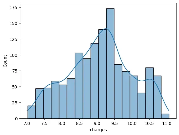
Log Transformation

4.2. Binary Encoding of Categorical Features

We will convert binary categorical columns (sex and smoker) into numeric format.

• **map() – Converts categories to 0/1
• Ensures compatibility with LightGBM, XGBoost and other gradient boosting frameworks Python `

df['sex'] = df['sex'].map({'male': 0, 'female': 1}) df['smoker'] = df['smoker'].map({'no': 0, 'yes': 1}) df.head()

`

**Output:

Binary Encoding

4.3. One-Hot Encoding Multi-class Features

We will one-hot encode the region column, converting it into separate binary columns.

• **pd.get_dummies() – Creates binary columns for each category
• Avoids ordinal bias that might be introduced with label encoding Python `

df = pd.concat([df, pd.get_dummies(df['region']).astype('int')], axis=1) df.drop(['Id', 'region'], inplace=True, axis=1) df.head()

`

**Output:

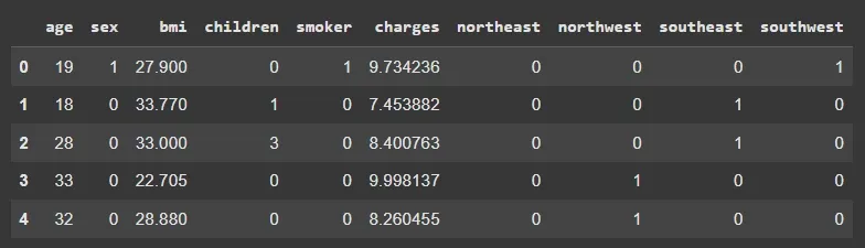
One-Hot Encoding

5. Splitting and Scaling Data

We will split the dataset into training and validation sets and scale the features.

• **train_test_split(): Splits features and target for training and validation
• **StandardScaler(): Standardizes features for consistency Python `

features = df.drop('charges', axis=1) target = df['charges']

X_train, X_val, Y_train, Y_val = train_test_split( features, target, test_size=0.25, random_state=2023 )

scaler = StandardScaler() X_train = scaler.fit_transform(X_train) X_val = scaler.transform(X_val)

`

6. Dataset Preparation for LightGBM

We will convert arrays into LightGBM dataset objects for training.

• **lgb.Dataset(): Prepares LightGBM-compatible datasets
• **reference: Ensures validation data is consistent with training data Python `

train_data = lgb.Dataset(X_train, label=Y_train) test_data = lgb.Dataset(X_val, label=Y_val, reference=train_data)

`

7. Regression Model Using LightGBM

We will define model parameters and train the LightGBM regressor.

• **objective: Defines task (regression)
• **metric: Evaluation metric (RMSE)
• **boosting_type: GBDT (Gradient Boosting Decision Trees)
• **num_leaves: Maximum leaf nodes per tree
• **learning_rate: Step size for boosting
• **feature_fraction: Fraction of features used per iteration
• **early_stopping_rounds: Stops training if no improvement Python `

params = { 'objective': 'regression', 'metric': 'rmse', 'boosting_type': 'gbdt', 'num_leaves': 31, 'learning_rate': 0.05, 'feature_fraction': 0.9 }

num_round = 100 bst = lgb.train(params, train_data, num_round, valid_sets=[ test_data], early_stopping_rounds=10)

`

**Output:

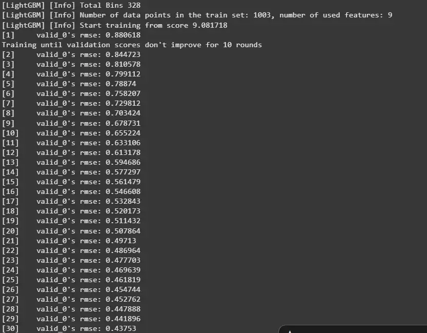
Training

8. Prediction and Evaluation

We will train the LightGBM regressor and evaluate its predictions.

• **LGBMRegressor(metric='rmse'): Initializes regressor
• **fit(): Trains the model
• **predict(): Generates predictions
• **np.sqrt(mse()): Computes RMSE Python `

model = LGBMRegressor(metric='rmse') model.fit(X_train, Y_train)

y_train = model.predict(X_train) y_val = model.predict(X_val)

print("Training RMSE: ", np.sqrt(mse(Y_train, y_train))) print("Validation RMSE: ", np.sqrt(mse(Y_val, y_val)))

`

**Output:

Training RMSE: 0.23318354433431218
Validation RMSE: 0.40587871797893876