Restricted Boltzmann Machine (original) (raw)

Last Updated : 2 Feb, 2026

A Boltzmann Machine is an unsupervised generative neural network that models data using energy-based states with fully connected bidirectional neurons. Due to this, full connectivity training is computationally expensive and inefficient in practice.

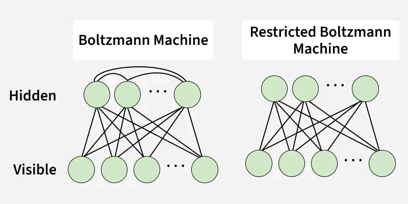
Boltzmann Machine Vs Restricted Boltzmann Machine

A Restricted Boltzmann Machine (RBM) is a simplified version of the Boltzmann Machine designed to make training feasible. It consists of a visible layer and a hidden layer with no connections allowed between neurons within the same layer. RBMs learn latent features from unlabeled data and are widely used for representation learning and dimensionality reduction.

• RBM is an unsupervised, generative, energy-based model that learns a probability distribution over input data.
• It has two layers only a visible (input) layer and a hidden (feature) layer with no intra-layer connections.
• RBMs are trained using Contrastive Divergence, which is an efficient approximation to maximum likelihood learning.
• They can discover latent features that explain correlations in the input data.
• RBMs are commonly used in feature learning, collaborative filtering, dimensionality reduction and as building blocks of Deep Belief Networks (DBNs).

How RBM Works

A Restricted Boltzmann Machine (RBM) is a generative stochastic neural network consisting of two layers a visible layer and a hidden layer. The term restricted means there are no connections within the same layer only between visible and hidden units.

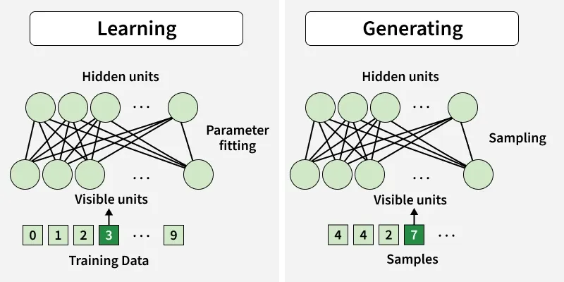
Parameter Learning vs. Sample Generation

The image shows the two phases of a Restricted Boltzmann Machine (RBM).

• During learning visible units receive training data and adjust weights with hidden units to model the data distribution.
• During generating the trained RBM uses sampling between hidden and visible units to produce new data samples similar to the training data.

RBM Architecture

• **Visible units (v): Represent the input data

v = (v_1, v_2, \dots, v_n)

• **Hidden units (h): Capture latent features

h = (h_1, h_2, \dots, h_m)

• **Weights (W): Connections between visible and hidden units. W_{ij} connects v_i \text{ and } h_j.
• **Biases: Visible bias {b_i} and hidden bias c_j

Energy Function

The RBM assigns an energy to each configuration of visible and hidden units:

E(v, h) = - \sum_{i=1}^{n} b_i v_i - \sum_{j=1}^{m} c_j h_j - \sum_{i=1}^{n} \sum_{j=1}^{m} v_i W_{ij} h_j

where

• v_i: state of visible unit i
• h_j: state of hidden unit j
• W_{ij}: weight between visible unit i and hidden unit j

Lower energy leads to higher probability.

Learning Process of Restricted Boltzmann Machine

The learning process of an RBM aims to reduce the reconstruction error. This is achieved by iteratively updating the weights so that the reconstructed data becomes closer to the original data distribution.

**1. Reconstruction Error

Reconstruction error is define by:

v^{(0)}-v^{(1)}

where

• v^{(0)}: original input (visible units)
• v^{(1)}: reconstructed input

The goal of learning is to minimize this error over successive training iterations by adjusting the weights W.

**2. Forward Pass

In the forward pass, we compute the probability of activating hidden units given the visible input v^{(0)}

P(h_j = 1 \mid v^{(0)}) = \sigma\!\left( c_j + \sum_{i=1}^{n} W_{ij} v^{(0)} \right)

**3. Backward Pass

In the backward pass, the RBM reconstructs the input using the hidden activations

P(v_i = 1 \mid h) = \sigma\!\left( b_i + \sum_{j=1}^{m} W_{ij} h_j \right)

**4. Joint Probability Distribution (Gibbs Distribution)

The joint probability of a visible–hidden configuration is:

P(v, h) = \frac{1}{Z} \exp\!\left(-E(v, h)\right)

where the partition function is:

Z = \sum_{v} \sum_{h} \exp\!\left(-E(v, h)\right)

**5. Generative Learning Perspective

RBM performs reconstruction, not classification or regression.

• It does not map inputs to labels
• Instead, it learns the probability distribution of the input data

Hence RBM is a generative model, unlike discriminative models used in classification.

**6. Error Minimization Using KL-Divergence

The difference between distributions represents the learning error and is measured using Kullback–Leibler (KL) divergence:

D_{KL}(p \parallel q) = \sum_{x} p(x) \log \frac{p(x)}{q(x)}

where

• p(x): true data distribution
• q(x): model’s reconstructed distribution

KL-divergence measures how much information is lost when q(x) approximates p(x)

**7. Weight Update Rule (Contrastive Divergence)

To reduce the KL-divergence RBM updates weights using:

\Delta W_{ij} = \eta \left( \langle v_i h_j \rangle_{\text{data}} - \langle v_i h_j \rangle_{\text{model}} \right)

where

• \eta: Learning Rate
• \langle v_i h_j \rangle_{\text{data}}: expectation from real data
• \langle v_i h_j \rangle_{\text{model}}: expectation from reconstructed data

Step By Step Implementation

In this code we train a Restricted Boltzmann Machine (RBM) on binarized MNIST images to learn feature representations then visualize reconstructed images from the RBM and generate new digit samples using Gibbs sampling

Step 1: Import Required Libraries

• numpy is used for numerical computations and matrix operations
• matplotlib is used for visualizing images and reconstructions
• mnist dataset is loaded from tensorflow Python `

import numpy as np import matplotlib.pyplot as plt from tensorflow.keras.datasets import mnist

`

Step 2: Load and Preprocess MNIST Dataset

• MNIST images are loaded as 28×28 grayscale images
• Images are flattened into 784-dimensional vectors
• Pixel values are normalized to the range [0, 1]
• Binary thresholding is applied for Bernoulli RBM Python `

(X_train, ), (, _) = mnist.load_data() X_train = X_train.reshape(-1, 784) / 255.0 X_train = (X_train > 0.5).astype(np.float32)

`

Step 3: Define the RBM Class Structure

• n_visible represents the number of visible units (pixels)
• n_hidden represents the number of hidden units (latent features)
• Weights are initialized with small random values
• Biases for visible and hidden layers are initialized to zero Python `

class RBM: def init(self, n_visible, n_hidden, lr=0.01): self.n_visible = n_visible self.n_hidden = n_hidden self.lr = lr self.W = np.random.normal(0, 0.01, (n_visible, n_hidden)) self.bv = np.zeros(n_visible) self.bh = np.zeros(n_hidden)

`

Step 4: Define Sigmoid Activation Function

• Sigmoid maps values into the range (0, 1)

• Output is interpreted as activation probability

• Used for both visible and hidden layers Python `

  def sigmoid(self, x): return 1 / (1 + np.exp(-x))

`

Step 5: Sampling from Probability Distribution

• RBM units are stochastic (binary)

• Bernoulli sampling converts probabilities into 0 or 1

• Enables Gibbs sampling behavior Python `

  def sample_prob(self, probs): return np.random.binomial(1, probs)

`

Step 6: Forward Pass

• Computes probability of hidden units given visible units

• Uses weight matrix and hidden bias

• Samples hidden activations Python `

  def forward(self, v): h_prob = self.sigmoid(np.dot(v, self.W) + self.bh) h_sample = self.sample_prob(h_prob) return h_prob, h_sample

`

Step 7: Backward Pass

• Reconstructs visible units from hidden activations

• Uses transpose of weight matrix

• Generates reconstructed input Python `

  def backward(self, h): v_prob = self.sigmoid(np.dot(h, self.W.T) + self.bv) v_sample = self.sample_prob(v_prob) return v_prob, v_sample

`

Step 8: Train RBM using Contrastive Divergence (CD-1)

• Original data is passed to the hidden layer (positive phase)

• Reconstructed data is generated (negative phase)

• Weights are updated using difference between data and reconstruction

• Reconstruction error is calculated using Mean Squared Error Python `

  def train(self, X, epochs=10, batch_size=64): n_samples = X.shape[0] for epoch in range(epochs): np.random.shuffle(X) epoch_error = 0 for i in range(0, n_samples, batch_size): v0 = X[i:i+batch_size] h0_prob, h0 = self.forward(v0) v1_prob, v1 = self.backward(h0) h1_prob, _ = self.forward(v1) self.W += self.lr * (np.dot(v0.T, h0_prob) - np.dot(v1.T, h1_prob)) / batch_size self.bv += self.lr * np.mean(v0 - v1, axis=0) self.bh += self.lr * np.mean(h0_prob - h1_prob, axis=0) epoch_error += np.mean((v0 - v1) ** 2) print(f"Epoch {epoch+1}/{epochs}, Reconstruction Error: {epoch_error:.4f}")

`

Step 9: Initialize and Train the RBM Model

• RBM is initialized with 784 visible and 256 hidden units
• Learning rate is set to 0.1
• Model is trained for 60 epochs using mini-batches Python `

rbm = RBM(n_visible=784, n_hidden=256, lr=0.1) rbm.train(X_train, epochs=60, batch_size=128)

`

**Output:

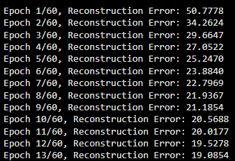
RBM Traning

Step 10: Visualize Input Reconstruction

• Displays original MNIST images
• Displays reconstructed images below them
• Helps evaluate how well RBM learned the data Python `

def plot_reconstruction(rbm, X, n=10): v = X[:n] _, h = rbm.forward(v) v_recon, _ = rbm.backward(h) plt.figure(figsize=(10, 4)) for i in range(n): plt.subplot(2, n, i+1) plt.imshow(v[i].reshape(28,28), cmap='gray') plt.axis('off') plt.subplot(2, n, i+n+1) plt.imshow(v_recon[i].reshape(28,28), cmap='gray') plt.axis('off') plt.show()

plot_reconstruction(rbm, X_train)

`

**Output:

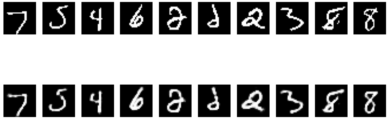
RBM MNIST reconstructions

This output shows the original MNIST images and their reconstructions generated by the RBM. It shows how well the Restricted Boltzmann Machine has learned to capture the underlying patterns of the digits.

Step 11: Generate New Samples using Gibbs Sampling

• Starts from random noise
• Alternates between visible and hidden layers
• Produces new digit-like samples learned from data distribution Python `

def generate_samples(rbm, steps=5000, n_samples=10): v = np.random.binomial(1, 0.5, (n_samples, rbm.n_visible)) for _ in range(steps): _, h = rbm.forward(v) _, v = rbm.backward(h) plt.figure(figsize=(10,2)) for i in range(n_samples): plt.subplot(1, n_samples, i+1) plt.imshow(v[i].reshape(28,28), cmap='gray') plt.axis('off') plt.show()

generate_samples(rbm)

`

**Output:

RBM output samples

This output shows new digit-like images generated entirely by the RBM from random noise. After multiple Gibbs sampling steps, the RBM produces samples that resemble the patterns it learned from the training data.

You can download full code from here

Types of Restricted Boltzmann Machines

1. **Binary Binary RBM: Standard RBM with binary visible and hidden units used for feature learning from binary or normalized data.
2. **Gaussian Binary RBM: Continuous visible units (Gaussian) and binary hidden units suitable for real valued data like images or audio.
3. **Bernoulli Gaussian RBM: Binary visible units and Gaussian hidden units; useful when latent features are continuous.
4. **Softmax RBM: Handles categorical/multinomial data using softmax activations; common in NLP tasks.
5. **Conditional RBM (CRBM): Conditions on extra context; ideal for sequential/temporal data like time-series or video.
6. **Convolutional RBM (ConvRBM): Uses weight sharing and local receptive fields; captures spatial hierarchies in images.
7. **Discriminative RBM: Incorporates labels for classification by modeling input features and targets together.
8. **Deep Belief Network (DBN): Stack of RBMs for hierarchical feature learning in deep architectures.

Applications

• **Feature Learning: RBMs automatically learn meaningful hidden representations from raw data, reducing the need for manual feature engineering.
• **Dimensionality Reduction: It can compress high dimensional data into lower dimensional latent features.
• **Collaborative Filtering: Widely used in recommender systems to predict user preferences.
• **Image Processing: Used for image reconstruction, denoising and pattern learning.
• **Pretraining Deep Networks: RBMs act as building blocks for Deep Belief Networks (DBNs), improving deep model initialization.
• **Anomaly Detection: It detect unusual patterns by modeling normal data distributions.

Advantages

• **Unsupervised Learning: RBMs do not require labeled data, making them useful when annotations are unavailable.
• **Generative Model: Capable of generating new data samples similar to the training data.
• **Efficient Training: Restricted structure allows faster training using Contrastive Divergence.
• **Feature Extraction: Learns latent features that capture important data patterns.
• **Probabilistic Interpretation: Based on probability distributions, enabling uncertainty modeling.

Limitations

• **Training Instability: RBMs are sensitive to hyperparameters like learning rate and number of hidden units.
• **Slow Convergence: Requires many epochs and Gibbs sampling steps to generate good samples.
• **Difficult to Scale: Computationally expensive for very large datasets.
• **Limited Interpretability: Learned features are often hard to interpret.
• **Evaluation Difficulty: Reconstruction error is only an approximate measure of model quality.