SelfTraining in SemiSupervised Learning (original) (raw)
Self-Training in Semi-Supervised Learning
Last Updated : 11 May, 2026
Self-training is a semi-supervised learning technique where a model is initially trained on a small labelled dataset and then iteratively refined using its own predictions.
- In each iteration, the model labels the most confident predictions on the unlabeled data, treating them as ground truth and includes them in the training set.
- This process continues until no significant improvement is achieved or all unlabeled data is used.
- Self-training is particularly useful when acquiring labelled data is costly or difficult, leveraging large amounts of unlabeled data to improve model performance.
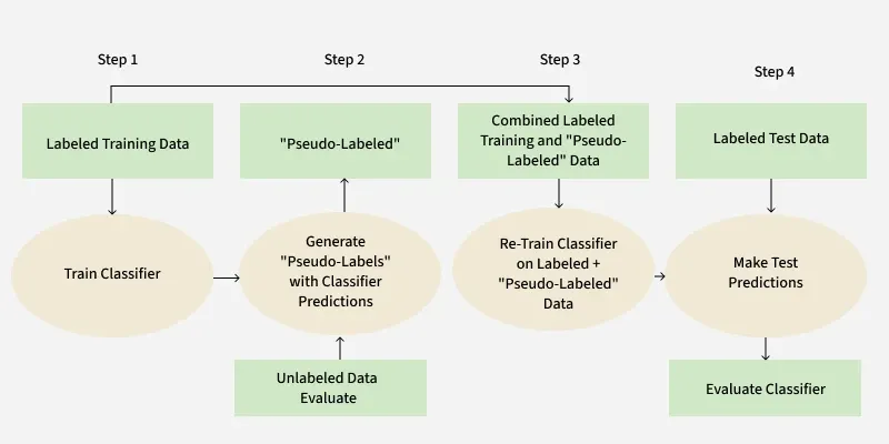
Steps of a Semi-Supervised Learning process using pseudo-labeling
Steps for Self-Training
- **Train on Labelled Data: Start with a model trained on a small labelled dataset.
- **Generate Pseudo-Labels: Use the trained model to predict labels for the unlabeled data. Filter these predictions by confidence thresholds (e.g., only accept predictions with high probabilities).
- **Augment Training Data: Add the pseudo-labeled samples to the original labeled dataset.
- **Iterative Refinement: Retrain the model on the augmented dataset. Repeat the process until the model's performance converges or a predefined number of iterations is reached.
Importance of Self-Training
- **Utilization of Unlabeled Data: Leverages large volumes of unlabeled data to improve model generalization.
- **Domain Independence: Works across various domains and tasks.
- **Efficiency: Can reduce the need for extensive manual labeling.
Self - Training Works in Practice
- A small subset of the data is labeled (e.g., 10% of the dataset).
- A logistic regression model is trained on this labeled data.
- The model is used to predict labels for the remaining unlabeled data.
- High-confidence predictions (e.g., those with probabilities above 95%) are added to the training set.
- The model is retrained with the expanded dataset, and the process repeats.
Implementation of Self-Training in Python
Below is a step-by-step implementation of **self-training using a **Random Forest classifier. The process involves training a model on a small set of labeled data, making predictions on unlabeled data, and iteratively adding high-confidence predictions to the labeled dataset.
**Step 1: Import Necessary Libraries
We begin by importing essential libraries required for dataset creation, model training, and evaluation. We use NumPy for numerical operations and dataset generation, along with machine learning tools from sklearn.
C++ `
import numpy as np
from sklearn.datasets import make_classification
from sklearn.metrics import accuracy_score
from sklearn.model_selection import train_test_split
`
**Step 2: Generate and Split the Dataset
A synthetic dataset is created with 1000 samples, 20 features, and 2 classes (binary classification). The first 100 samples are treated as labeled data, while the remaining 900 samples are considered unlabeled, containing only features without labels. The unlabeled data is further split into a separate test set to evaluate the model later.
C++ `
Generate synthetic dataset
X, y = make_classification(n_samples=1000, n_features=20, n_classes=2, random_state=42)
Split into labeled and unlabeled data
X_labeled, y_labeled = X[:100], y[:100] # First 100 samples are labeled X_unlabeled, X_test, y_unlabeled, y_test = train_test_split(X[100:], y[100:], test_size=0.2, random_state=42)
`
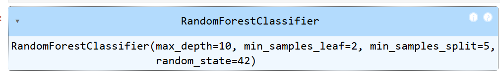
**Step 3: Initialize and Train the Model
Random Forest Classifier is initialized, an ensemble-based model that constructs multiple decision trees during training. It is known for its robustness in classification tasks and ability to handle non-linearity effectively.
C++ `
from sklearn.ensemble import RandomForestClassifier
Initialize the classifier with additional hyperparameters
model = RandomForestClassifier( n_estimators=100, # Number of trees in the forest max_depth=10, # Maximum depth of each tree min_samples_split=5, # Minimum samples required to split a node min_samples_leaf=2, # Minimum samples required in each leaf node max_features="sqrt", # Number of features considered for best split bootstrap=True, # Use bootstrap sampling random_state=42 )
Train the model on the labeled data
model.fit(X_labeled, y_labeled)
`
**Output:
Output
**Step 4: Perform Self-Training Iterations
Self-training process is performed over five iterations.
- In each iteration, the model generates pseudo-labels for the unlabeled data and calculates confidence scores for its predictions.
- Samples with high-confidence predictions are added to the labeled dataset, while those with lower confidence remain unlabeled.
- The model is then retrained on the expanded labeled dataset, progressively improving its performance. C++ `
for _ in range(5): # Run 5 iterations pseudo_labels = model.predict(X_unlabeled) # Generate pseudo-labels pseudo_probabilities = model.predict_proba(X_unlabeled).max(axis=1) # Get confidence scores
threshold = 0.9  # Confidence threshold for pseudo-labeling
confident_indices = np.where(pseudo_probabilities > threshold)[0]  # Identify confident samples

# Add confident pseudo-labeled samples to the labeled dataset
X_labeled = np.vstack((X_labeled, X_unlabeled[confident_indices]))
y_labeled = np.hstack((y_labeled, pseudo_labels[confident_indices]))

# Remove pseudo-labeled samples from the unlabeled set
X_unlabeled = np.delete(X_unlabeled, confident_indices, axis=0)

# Retrain the model with the expanded labeled dataset
model.fit(X_labeled, y_labeled)
`
**Step 5: Evaluate the Model
Once self-training is complete, the model is evaluated on a separate test set. The accuracy score is computed to measure the effectiveness of the self-training approach. This step ensures that the model generalizes well to unseen data.
C++ `
Predict labels on the test dataset
y_pred = model.predict(X_test)
Print accuracy
print("Final Model Accuracy on Test Data:", accuracy_score(y_test, y_pred))
`
**Output
Accuracy: 0.875
Complete Code:
Python `
import numpy as np from sklearn.datasets import make_classification from sklearn.ensemble import RandomForestClassifier from sklearn.metrics import accuracy_score from sklearn.model_selection import train_test_split
Step 1: Generate and split dataset
X, y = make_classification(n_samples=1000, n_features=20, n_classes=2, random_state=42) X_labeled, y_labeled = X[:100], y[:100] X_unlabeled, X_test, y_unlabeled, y_test = train_test_split(X[100:], y[100:], test_size=0.2, random_state=42)
Step 2: Initialize and train the model
model = RandomForestClassifier( n_estimators=100, max_depth=10, min_samples_split=5, min_samples_leaf=2, max_features="sqrt", bootstrap=True, random_state=42 ) model.fit(X_labeled, y_labeled)
Step 3: Perform self-training iterations
confidence_threshold = 0.9
for iteration in range(5): print(f"Iteration {iteration + 1}: Labeled Samples - {len(y_labeled)}")
pseudo_labels = model.predict(X_unlabeled)
pseudo_probabilities = model.predict_proba(X_unlabeled).max(axis=1)
confident_indices = np.where(pseudo_probabilities > confidence_threshold)[0]

# Update labeled dataset
X_labeled = np.vstack((X_labeled, X_unlabeled[confident_indices]))
y_labeled = np.hstack((y_labeled, pseudo_labels[confident_indices]))

# Remove pseudo-labeled samples from the unlabeled set
X_unlabeled = np.delete(X_unlabeled, confident_indices, axis=0)

# Retrain the model
model.fit(X_labeled, y_labeled)
print(f"Final number of labeled samples: {len(y_labeled)}")
Step 4: Evaluate the final model
y_pred = model.predict(X_test) print("Final Model Accuracy on Test Data:", accuracy_score(y_test, y_pred))
`
**Output
Accuracy: 0.875
The model achieves an accuracy of 87.5% on the test set after 5 iterations of self-training. This means that the model correctly classified 87.5 percent of the samples in the test set.
Comparison with Other Semi-Supervised Learning Methods
- **Self-Training vs. Co-Training: Co-Training uses two models with complementary views of the data, while Self-Training uses a single model.
- **Self-Training vs. Graph-Based Methods: Graph-based methods rely on data structure and relationships, while Self-Training operates directly on feature representations.
- **Self-Training vs. Generative Models: Generative models (e.g., Variational Autoencoders) focus on learning data distributions, whereas Self-Training directly enhances classification tasks.
Applications
- **Natural Language Processing (NLP): Text classification, sentiment analysis, and question answering.
- **Computer Vision: Image recognition and object detection.
- **Healthcare: Medical diagnosis and imaging analysis.
- **Speech Processing: Speaker recognition and voice activity detection.
- Benefits and Challenges
Benefits
- **Cost Efficiency: Requires minimal labeled data.
- **Flexibility: Can be applied to various models and tasks.
- **Simplicity: Easy to implement with standard machine learning libraries.
Challenges
- **Error Amplification: Incorrect pseudo-labels may degrade performance over iterations.
- **Confidence Thresholding: Selecting a proper confidence threshold is non-trivial.
- **Imbalanced Datasets: Models may propagate bias in imbalanced datasets.