Singular Value Decomposition (SVD) (original) (raw)
Last Updated : 5 Jul, 2025
Singular Value Decomposition (SVD) is a factorization method in linear algebra that decomposes a matrix into three other matrices, providing a way to represent data in terms of its singular values.
SVD helps you split that table into three parts:
- **U: This part tells you about the people (like their general preferences).
- **Σ: This part shows how important each factor is (how much each rating matters).
- **Vᵀ: This part tells you about the products (how similar they are to each other)
Lets understand this with help of an example: Suppose you have a small table of people’s ratings for two movies,
| Name | Movie 1 Rating | Movie 2 Rating |
|---|---|---|
| Amit | 5 | 3 |
| Sanket | 4 | 2 |
| Harsh | 2 | 5 |
- SVD breaks this table into three smaller parts: one that shows people’s preferences, one that shows the importance of each movie, and one that shows how similar the movies are to each other
- Mathematically, the SVD of a matrix A (of size m \times n) is represented as: A = U \Sigma V^T
Here:
- U: An m \times m orthogonal matrix whose columns are the left singular vectors of A.
- \Sigma: A diagonal m \times n matrix containing the singular values of A in descending order.
- V^T: The transpose of an n \times n orthogonal matrix, where the columns are the right singular vectors of A.
How to perform Singular Value Decomposition
To perform Singular Value Decomposition (SVD) for the matrix A = \begin{bmatrix} 3 & 2 & 2 \\ 2 & 3 & -2 \end{bmatrix}, let's break it down step by step.
**Step 1: Compute A A^T
First, we need to calculate the matrix A A^T (where A^T is the transpose of matrix A):
A = \begin{bmatrix} 3 & 2 & 2 \\ 2 & 3 & -2 \end{bmatrix}A^T = \begin{bmatrix} 3 & 2 \\ 2 & 3 \\ 2 & -2 \end{bmatrix}
Now, compute A A^T:
A A^T = \begin{bmatrix} 3 & 2 & 2 \\ 2 & 3 & -2 \end{bmatrix} \cdot \begin{bmatrix} 3 & 2 \\ 2 & 3 \\ 2 & -2 \end{bmatrix} = \begin{bmatrix} 17 & 8 \\ 8 & 17 \end{bmatrix}
**Step 2: Find the Eigenvalues of A A^T
To find the eigenvalues of A A^T, we solve the characteristic equation:
\det(A A^T - \lambda I) = 0
\det \begin{bmatrix} 17 - \lambda & 8 \\ 8 & 17 - \lambda \end{bmatrix} = 0
(\lambda - 25)(\lambda - 9) = 0Thus, the eigenvalues are \lambda_1 = 25 and \lambda_2 = 9. These eigenvalues correspond to the singular values \sigma_1 = 5 and \sigma_2 = 3, since the singular values are the square roots of the eigenvalues.
Step 3: Find the Right Singular Vectors (Eigenvectors of A^T A)
Next, we find the eigenvectors of A^T A for \lambda = 25 and \lambda = 9.
For \lambda = 25:
Solve (A^T A - 25I) v = 0:
A^T A - 25I = \begin{bmatrix} -12 & 12 & 2 \\ 12 & -12 & -2 \\ 2 & -2 & -17 \end{bmatrix}Row-reduce this matrix to:
\begin{bmatrix} 1 & -1 & 0 \\ 0 & 0 & 1 \\ 0 & 0 & 0 \end{bmatrix}The eigenvector corresponding to \lambda = 25 is:
v_1 = \begin{bmatrix} \frac{1}{\sqrt{2}} \\ \frac{1}{\sqrt{2}} \\ 0 \end{bmatrix}For \lambda = 9:
Solve (A^T A - 9I) v = 0:
The eigenvector corresponding to \lambda = 9 is:
v_2 = \begin{bmatrix} \frac{1}{\sqrt{18}} \\ \frac{-1}{\sqrt{18}} \\ \frac{4}{\sqrt{18}} \end{bmatrix}For the third eigenvector v_3:
Since v3 must be perpendicular to v_1 and v_2, we solve the system v_1^T v_3 = 0 and v_2^T v_3 = 0, leading to:
v_3 = \begin{bmatrix} \frac{2}{3} \\ \frac{-2}{3} \\ \frac{-1}{3} \end{bmatrix}
**Step 4: Compute the Left Singular Vectors (Matrix U)
To compute the left singular vectors U, we use the formula u_i = \frac{1}{\sigma_i} A v_i. This results in:
U = \begin{bmatrix} \frac{1}{\sqrt{2}} & \frac{1}{\sqrt{2}} \\ \frac{1}{\sqrt{2}} & \frac{-1}{\sqrt{2}} \end{bmatrix}
**Step 5: Final SVD Equation
Finally, the Singular Value Decomposition of matrix A is:
A = U \Sigma V^TWhere:
U = \begin{bmatrix} \frac{1}{\sqrt{2}} & \frac{1}{\sqrt{2}} \\ \frac{1}{\sqrt{2}} & \frac{-1}{\sqrt{2}} \end{bmatrix}\Sigma = \begin{bmatrix} 5 & 0 & 0 \\ 0 & 3 & 0 \end{bmatrix}
V = \begin{bmatrix} \frac{1}{\sqrt{2}} & \frac{1}{\sqrt{2}} & 0 \\ \frac{1}{\sqrt{18}} & \frac{-1}{\sqrt{18}} & \frac{4}{\sqrt{18}} \\ \frac{2}{3} & \frac{-2}{3} & \frac{1}{3} \end{bmatrix}
Thus, the SVD of matrix A is:
A = \begin{bmatrix} \frac{1}{\sqrt{2}} & \frac{1}{\sqrt{2}} \\ \frac{1}{\sqrt{2}} & \frac{-1}{\sqrt{2}} \end{bmatrix} \begin{bmatrix} 5 & 0 & 0 \\ 0 & 3 & 0 \end{bmatrix} \begin{bmatrix} \frac{1}{\sqrt{2}} & \frac{1}{\sqrt{2}} & 0 \\ \frac{1}{\sqrt{18}} & \frac{-1}{\sqrt{18}} & \frac{4}{\sqrt{18}} \\ \frac{2}{3} & \frac{-2}{3} & \frac{1}{3} \end{bmatrix}
This is the Result SVD matrix of matrix A.
Applications of Singular Value Decomposition (SVD)
1. **Calculation of Pseudo-Inverse (Moore-Penrose Inverse)
- The pseudo-inverse is a generalization of the matrix inverse, applicable to non-invertible matrices like low-rank matrices. For an invertible matrix, it equals the inverse.
- Denoted as M^+ , it is calculated using the SVD M = U\Sigma V^T , where U and V are orthogonal matrices of left and right singular vectors, and \Sigma is a diagonal matrix of singular values.
- Pseudo-inverse formula: M^+ = V\Sigma^{-1}U^T , where \Sigma^{-1} inverts non-zero singular values.
2. **Solving a Set of Homogeneous Linear Equations
- For M x = b , if b = 0, use SVD to choose a column of V associated with a zero singular value.
- If b \neq 0, solve by multiplying both sides by M^+ : x = M^+ b.
3. **Rank, Range, and Null Space
The rank, range, and null space of a matrix M can be derived from its SVD.
- **Rank: The rank of matrix M is the number of non-zero singular values in \Sigma.
- **Range: The range of matrix M is the span of the left singular vectors in matrix U corresponding to the non-zero singular values.
- **Null Space: The null space of matrix M is the span of the right singular vectors in matrix V corresponding to the zero singular values.
4. **Curve Fitting Problem
Singular Value Decomposition can be used to minimize the least square error in the curve fitting problem. By approximating the solution using the pseudo-inverse, we can find the best-fit curve to a given set of data points.
5. **Applications in Digital Signal Processing (DSP) and Image Processing
- **Digital Signal Processing: SVD can be used to analyze signals and filter noise.
- **Image Processing: SVD is used for image compression and denoising. It helps in reducing the dimensionality of image data by preserving the most significant singular values and discarding the rest.
Implementation of Singular Value Decomposition (SVD)
In this code, we will try to calculate the Singular value decomposition using Numpy and Scipy. We will be calculating SVD, and also performing pseudo-inverse. In the end, we can apply SVD for compressing the image
Python `
from skimage.color import rgb2gray from skimage import data import matplotlib.pyplot as plt import numpy as np from scipy.linalg import svd
X = np.array([[3, 3, 2], [2, 3, -2]]) print(X)
U, singular, V_transpose = svd(X)
print("U: ", U) print("Singular array", singular) print("V^{T}", V_transpose)
singular_inv = 1.0 / singular s_inv = np.zeros(X.shape) s_inv[0][0] = singular_inv[0] s_inv[1][1] = singular_inv[1] M = np.dot(np.dot(V_transpose.T, s_inv.T), U.T) print(M)
cat = data.chelsea() plt.imshow(cat)
gray_cat = rgb2gray(cat)
U, S, V_T = svd(gray_cat, full_matrices=False) S = np.diag(S) fig, ax = plt.subplots(5, 2, figsize=(8, 20))
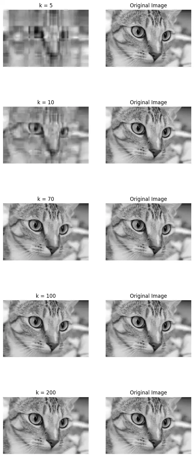
curr_fig = 0 for r in [5, 10, 70, 100, 200]: cat_approx = U[:, :r] @ S[0:r, :r] @ V_T[:r, :] ax[curr_fig][0].imshow(cat_approx, cmap='gray') ax[curr_fig][0].set_title("k = " + str(r)) ax[curr_fig, 0].axis('off') ax[curr_fig][1].set_title("Original Image") ax[curr_fig][1].imshow(gray_cat, cmap='gray') ax[curr_fig, 1].axis('off') curr_fig += 1 plt.show()
`
**Output:
[[ 3 3 2]
[ 2 3 -2]]
U: [[-0.7815437 -0.6238505]
[-0.6238505 0.7815437]]
Singular array [5.54801894 2.86696457]
V^{T} [[-0.64749817 -0.7599438 -0.05684667]
[-0.10759258 0.16501062 -0.9804057 ]
[-0.75443354 0.62869461 0.18860838]]
Inverse
array([[ 0.11462451, 0.04347826],
[ 0.07114625, 0.13043478],
[ 0.22134387, -0.26086957]])
Output
The output consists of subplots showing the compressed image for different values of r (5, 10, 70, 100, 200), where r represents the number of singular values used in the approximation. As the value of r increases, the compressed image becomes closer to the original grayscale image of the cat, with smaller values of r leading to more blurred and blocky images, and larger values retaining more details.