Spectral Clustering (original) (raw)
Last Updated : 3 Apr, 2026
Spectral Clustering is an unsupervised learning technique used to group data points based on their similarity. It uses concepts from graph theory and linear algebra to transform data into a space where clustering becomes easier.
- Works well for non-linear and complex shapes
- Uses concepts from linear algebra (eigenvalues & eigenvectors)
- Converts data into a graph structure (nodes and edges)
Types of Spectral Clustering
- **Unnormalized Spectral Clustering: Uses the similarity values directly to group data points without any adjustment but it may not perform well when the data is uneven.
- **Normalized Spectral Clustering: Adjusts the similarity values before clustering, which helps in getting better and more balanced clusters in most real-world datasets.
- **Random Walk Spectral Clustering: Groups data points based on how strongly they are connected to each other in the graph.
Key Concepts
It explains how data is represented and transformed so that clusters can be identified more easily. The main concepts involved are:
1. Similarity Matrix (W)
The matrix which represents how similar two data points are. It measures the relationship between every pair of points based on distance.
W_{ij} = e^{-\frac{||x_i - x_j||^2}{2\sigma^2}}
- If two points are close then value is high
- If far then value is low
This forms a graph where points are nodes and similarity is edges.
2. Degree Matrix (D)
Degree matrix represents the total connection strength of each data point. It is formed by summing all similarity values for a given point.
D_{ii} = \sum_{j} W_{ij}
- Diagonal matrix
- Shows how strongly each point is connected
3. Graph Laplacian (L)
This matrix identifies the structure of the graph. It is obtained by subtracting the similarity matrix from the degree matrix.
L = D - W
- Core matrix in Spectral Clustering
- Helps identify connected groups
4. Eigenvalues & Eigenvectors
These are mathematical tools used to extract important patterns from the data. They help transform the data into a new space where clusters become clearer.
- Used for dimensionality reduction
- Makes clusters easier to separate
Working
The steps involved in Spectral Clustering are as follows:
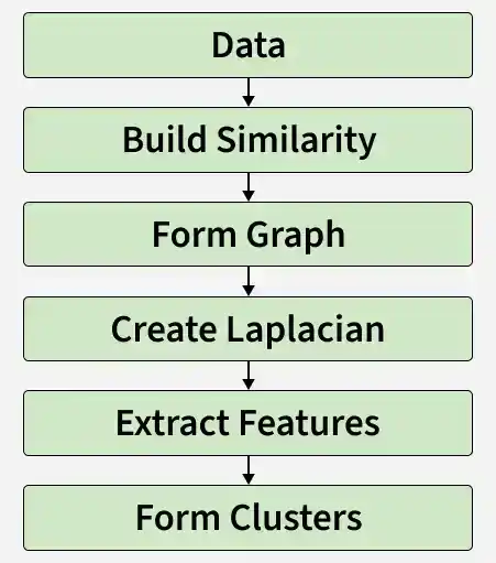
Working of Spectral Clustering
**Step 1: Converting data into a graph structure where
- Each point is a node
- Similar points are connected (strong connection = similar points)
**Step 2: Now,Instead of looking at raw data, we study this network structure.
**Step 3: The Laplacian matrix combines similarity and connection information to reveal the structure of the data.
- Strong connections (same cluster)
- Weak connections (different clusters)
**Step 4: Eigenvectors are then used to rearrange the data into a new form.
**Step 5: Here, data is transformed into a new lower-dimensional space where points from same cluster move closer
**Step 6: We apply K - Means algorithm where clusters become easy to detect.
Implementation
Step 1: Importing Libraries
Importing libraries like
- NumPy for numerical operations
- Matplotlib for visualization
- Scikit-learn modules for dataset generation and Spectral Clustering Python `
import numpy as np import matplotlib.pyplot as plt from sklearn.datasets import make_moons from sklearn.cluster import SpectralClustering
`
Step 2: Creating a Dataset
In this step, we create a sample non-linear dataset to apply Spectral Clustering.
Python `
X, _ = make_moons(n_samples=300, noise=0.05)
`
Step 3: Visualizing the Original Dataset
Now, we plot the dataset to understand its distribution. It helps understand actual structure of data.
Python `
plt.scatter(X[:, 0], X[:, 1])
plt.title("Original Data")
plt.show()
`
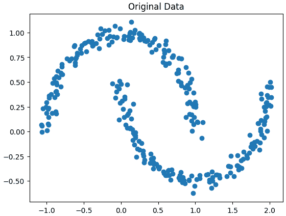
Raw Dataset before Clustering
Step 4: Building a Spectral Clustering Model
Here, we build the Spectral Clustering model by setting parameters such as the number of clusters and the method used to compute similarity between data points.
- n_clusters is number of clusters
- affinity is how similarity is computed
- Uses nearest neighbors to build graph Python `
model = SpectralClustering( n_clusters=2, affinity='nearest_neighbors', n_neighbors=15 )
`
Step 5: Training the model
This step involves fitting the model to the data and grouping points into clusters. This is done using fit_predict() which fits the model and returns the cluster labels.
Python `
labels = model.fit_predict(X)
`
Step 6: Visualizing the Clustered Output
The clustered data is visualized to show the final grouping of data points. Different colors are used to represent different clusters****.**
Python `
plt.scatter(X[:, 0], X[:, 1], c=labels)
plt.title("Spectral Clustering")
plt.show()
`
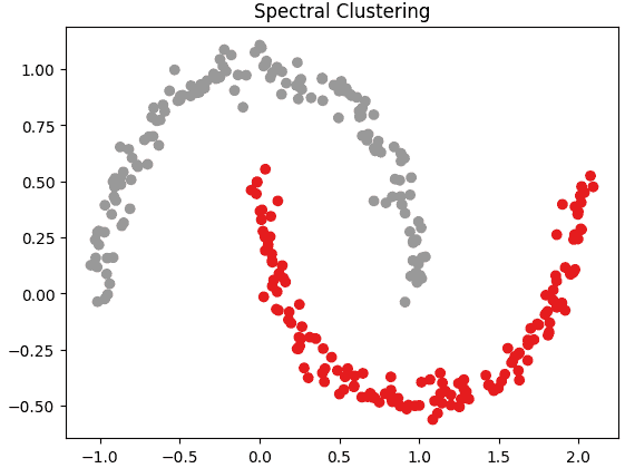
Spectral Clustering Result
Step 7: Applying K-Means algorithm for comparison
Here, we apply K-Means algorithm to the same dataset for comparison. This helps in understanding how Spectral Clustering performs better than K-Means algorithm on non-linear data.
Python `
from sklearn.cluster import KMeans
kmeans = KMeans(n_clusters=2, random_state=42) k_labels = kmeans.fit_predict(X)
plt.figure(figsize=(10,4))
plt.subplot(1,2,1) plt.scatter(X[:, 0], X[:, 1], c=labels) plt.title("Spectral Clustering")
plt.subplot(1,2,2) plt.scatter(X[:, 0], X[:, 1], c=k_labels) plt.title("K-Means Clustering")
plt.show()
`
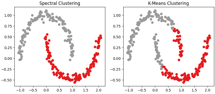
Spectral Clustering vs K-Means Clustering
The complete source code can be accessed here.
Applications
- Image segmentation helps in separating different objects or regions in an image based on pixel similarity.
- Social network analysis identifies communities or groups of closely connected users.
- Recommendation systems group similar users or items to provide better recommendations.
- Bioinformatics helps in clustering genes or proteins based on similarity in biological data.
- Pattern recognition is useful in identifying patterns and structures in complex datasets.
Limitations
- Takes more time to run due to complex calculations
- Not suitable for very large datasets
- High memory usage
- Requires proper parameter selection (like number of clusters, neighbors).