StandardScaler, MinMaxScaler and RobustScaler techniques ML (original) (raw)
Last Updated : 24 Oct, 2025
In machine learning value of features may have different ranges and units. This variation can impact negatively on the performance of algorithms like KNN, SVM or Logistic Regression. To avoid this issue **feature scaling is used to standardize data. In this article, we’ll see three commonly used scaling techniques:
1. **StandardScaler
**StandardScaler is a feature scaling technique which follows**Standard Normal Distribution (SND) and is used to standardize the values of numeric features. It transforms data so that the mean becomes 0 and the standard deviation becomes 1. It’s ideal for algorithms like SVM, logistic regression or neural networks that assume data is normally distributed
It subtracts mean of the data and divides by the standard deviation. This centers the data around zero and standardizes variability.
X_{\text{scaled}} = \frac{X - \mu}{\sigma}
Where:
- X is the original value,
- μ is the mean of the feature,
- σ is the standard deviation.
**Advantages
- It handles features with different units effectively.
- It reduces impact of outliers without completely removing them.
**Disadvantages
- It is sensitive to outliers and extreme values can skew mean and standard deviation which leads to poor scaling.
- It is not ideal for non-normal distributions.
2. MinMaxScaler
**MinMaxScaler scales all data features in range _[0, 1] or else in range _[-1, 1] if there are negative values are present in the dataset. Use it when our data does not follow a normal distribution or when we need scaled data for algorithms like decision trees, k-nearest neighbors or support vector machines. It gives best results when outliers are minimal or absent as it is sensitive to extreme values.
It scales data to a fixed range (typically [0, 1]) by subtracting minimum value and dividing by the range (max - min) which ensures all feature values lies within specified range.
X_{\text{scaled}} = \frac{X - X_{\min}}{X_{\max} - X_{\min}}
Where:
- X is the original value
- X_{\min} is the minimum value of the feature
- X_{\max}is the maximum value of the feature
**Advantages
- It ensures that all features have same scale.
- It is simple and easy to interpret.
**Disadvantages
- It is sensitive to outliers and the extreme values can distort scaling which makes most data points cluster near 0 or 1.
- Fixed range limits flexibility for datasets with changing scales.
3. RobustScaler
RobustScaler reduces the impact of outliers by scaling data using median and interquartile range (IQR) which makes it fit to extreme values. We use it when our data contains many outliers and we need to maintain relative distances between non-outlier data points or we’re working with algorithms which are sensitive to extreme values.
It subtracts median of data and divides by interquartile range (IQR) which helps in reducing the effect of outliers while maintaining distribution of non-outlier values. The median and IQR are stored during fitting so they can be applied to future data using the transform method.
X_{\text{scaled}} = \frac{X - Median(X)}{Q_3 - Q_1}
Where:
- X is the original value
- Median(X) is the Q_2 or the median quartile (50th percentile)
- Q_1 is the first quartile (25th percentile)
- Q_3 is the third quartile (75th percentile)
**Advantages
- It is resistant to outliers.
- It maintains the structure of data and it is better than MinMaxScaler in the presence of extreme values.
**Disadvantages
- This may not perform well when data is highly skewed.
- It is less interpretable compared to MinMaxScaler.
**Implementing Comparison between StandardScaler, MinMaxScaler and RobustScaler.
We will be using **Pandas, **Numpy, **Matplotlib****,** Scikit learnand **Seaborn libraries for this implementation.
- **np.random.normal: This is used to generate random values from a normal distribution, it is responsible for generating the data in x1 and x2.
- **scaler = preprocessing.RobustScaler(): This creates an example of RobustScaler to scale data by using median and interquartile range.
- **scaler = preprocessing.StandardScaler(): This creates an example of StandardScaler to scale data by removing mean and scaling to unit variance.
- **scaler = preprocessing.MinMaxScaler(): This creates an example of MinMaxScaler to scale data to a specified range [0, 1]. Python `
import pandas as pd import numpy as np from sklearn import preprocessing import matplotlib import matplotlib.pyplot as plt import seaborn as sns % matplotlib inline matplotlib.style.use('fivethirtyeight') x = pd.DataFrame({ 'x1': np.concatenate([np.random.normal(20, 2, 1000), np.random.normal(1, 2, 25)]), 'x2': np.concatenate([np.random.normal(30, 2, 1000), np.random.normal(50, 2, 25)]), }) np.random.normal
scaler = preprocessing.RobustScaler() robust_df = scaler.fit_transform(x) robust_df = pd.DataFrame(robust_df, columns=['x1', 'x2'])
scaler = preprocessing.StandardScaler() standard_df = scaler.fit_transform(x) standard_df = pd.DataFrame(standard_df, columns=['x1', 'x2'])
scaler = preprocessing.MinMaxScaler() minmax_df = scaler.fit_transform(x) minmax_df = pd.DataFrame(minmax_df, columns=['x1', 'x2'])
fig, (ax1, ax2, ax3, ax4) = plt.subplots(ncols=4, figsize=(20, 5)) ax1.set_title('Before Scaling') sns.kdeplot(x['x1'], ax=ax1, color='r') sns.kdeplot(x['x2'], ax=ax1, color='b') ax2.set_title('After Robust Scaling') sns.kdeplot(robust_df['x1'], ax=ax2, color='red') sns.kdeplot(robust_df['x2'], ax=ax2, color='blue') ax3.set_title('After Standard Scaling') sns.kdeplot(standard_df['x1'], ax=ax3, color='black') sns.kdeplot(standard_df['x2'], ax=ax3, color='g') ax4.set_title('After Min-Max Scaling') sns.kdeplot(minmax_df['x1'], ax=ax4, color='black') sns.kdeplot(minmax_df['x2'], ax=ax4, color='g') plt.show()
`
Output:
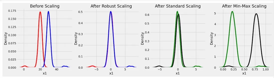
Comparison in all three Scaling Techniques
Output shows how three scalers transform two features i.e x1 and x2. Before scaling, features have different ranges and skewed distributions.
- **RobustScaler uses median and IQR to handle outliers while maintaing data's shape.
- **StandardScaler adjusts data to have a mean of 0 and standard deviation of 1 but it is sensitive to outliers.
- **MinMaxScaler scales data to a fixed range ([0, 1]) but extreme values can effect results. Each scaler works best in specific situations:
Choosing right scaler depends on characteristics of data and algorithm being used. By understanding their strengths and limitations we can preprocess data effectively and build stronger machine learning models.