Time Series using LightGBM (original) (raw)

Last Updated : 23 Jul, 2025

Time series forecasting is a method used to predict future values based on past data points collected over time. This type of data appears in many real-life applications such as predicting sales, stock prices, weather conditions or traffic patterns. One tool for time series forecasting is LightGBM which is a fast and efficient machine learning algorithm developed by Microsoft. It stands for Light Gradient Boosting Machine and is based on gradient boosting which builds a strong prediction model from many smaller models called decision trees.

What is Time Series Data?

Time series data is a sequence of observations collected over time usually in regular intervals like:

• Daily stock prices
• Hourly temperature readings
• Monthly electricity usage

The key characteristic of time series data is that order matters. The value at time t depends on what happened before time t. For example, if we are forecasting tomorrow’s weather we would use the data from today, yesterday and the days before that.

Why use LightGBM for Time Series

LightGBM is a great choice for time series forecasting because it handles missing data well, works efficiently with large datasets and supports a wide variety of features such as weather conditions, holidays and special events. It also allows the use of custom loss functions, which can be helpful when optimizing for specific forecasting goals. One of LightGBM’s biggest advantages is its fast training and prediction speed, making it suitable for real-time or large-scale forecasting tasks. Although it's not specifically designed for time series, with the right feature engineering and data transformation, LightGBM can deliver highly accurate and reliable forecasts.

Preparing Data for LightGBM

Since LightGBM is not built for time series, we need to **manually add features that represent the time structure. Here’s how to prepare time series data:

1. Create Lag Features

Lag features represent past values of the series. For example:

• lag\_1 = value at time t-1
• lag\_2 = value at time t-2

This helps the model understand how the current value depends on the past.

Python `

import pandas as pd import numpy as np

Create sample time series data

date_range = pd.date_range(start='2022-01-01', periods=100, freq='D') values = np.random.randn(100) # random values

Create the DataFrame

df = pd.DataFrame({'date': date_range, 'value': values})

df['lag_1'] = df['value'].shift(1) df['lag_2'] = df['value'].shift(2)

`

2. Create Rolling Statistics

Rolling features include moving averages or standard deviations over a time window:

Python `

df['rolling_mean_3'] = df['value'].rolling(3).mean() df['rolling_std_3'] = df['value'].rolling(3).std()

`

These features show trends or seasonality.

3. Add Date-Based Features

You can extract useful features from the date, such as:

• Day of the week (Monday, Tuesday, etc.)
• Month
• Is it a weekend? Python `

df['day_of_week'] = df['date'].dt.dayofweek df['month'] = df['date'].dt.month df['is_weekend'] = df['day_of_week'].isin([5,6]).astype(int)

`

4. Remove Missing Values

Because lag and rolling features create NaN values in the beginning, you’ll need to drop them:

Python `

df = df.dropna()

`

Building a Time Series Model with LightGBM

Now that the data is ready, we can build the model.

Step 1: Installing LightGBM

You can install it using pip:

Python `

pip install lightgbm

`

Step 2: Splitting Data

For time series we must not shuffle the data. Instead split it by time:

Python `

train = df[df['date'] < '2022-04-01'] test = df[df['date'] >= '2022-04-01']

`

Step 3: Defining Features and Target

Python `

features = ['lag_1', 'lag_2', 'rolling_mean_3', 'day_of_week', 'month', 'is_weekend'] target = 'value'

X_train = train[features] y_train = train[target]

X_test = test[features] y_test = test[target]

`

Step 4: Training LightGBM Model

Python `

import lightgbm as lgb

model = lgb.LGBMRegressor() model.fit(X_train, y_train)

`

Step 5: Making Predictions

Python `

predictions = model.predict(X_test)

`

Evaluating the Model

To check how good your model is, use metrics like:

• **MAE (Mean Absolute Error): average of absolute differences between predicted and actual values.
• **RMSE (Root Mean Square Error): square root of the average of squared errors.

Example:

Python `

from sklearn.metrics import mean_absolute_error, mean_squared_error import numpy as np

mae = mean_absolute_error(y_test, predictions) rmse = np.sqrt(mean_squared_error(y_test, predictions))

print(f"MAE: {mae}") print(f"RMSE: {rmse}")

`

**Output:

MAE: 0.3466166706030231
RMSE: 0.4253669139921471

Plotting the Forecast

It’s always helpful to see how predictions look compared to actual values:

Python `

import matplotlib.pyplot as plt

plt.figure(figsize=(6, 4)) plt.plot(test['date'], y_test, label='Actual') plt.plot(test['date'], predictions, label='Predicted') plt.xticks(test['date'], rotation=45)

plt.xlabel("Date") plt.ylabel("Value") plt.title("Time Series Forecasting with LightGBM") plt.legend() plt.tight_layout() plt.grid(True) plt.show()

`

**Output:

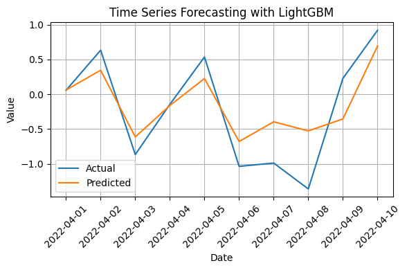
Time Series Forecasting with LightGBM

Limitations of LightGBM for Time Series

While LightGBM is a great tool, it has some limitations for time series:

• It does not model time directly you have to create time-based features yourself.
• It cannot forecast multiple steps ahead easily. For that you need to predict one step at a time and feed it back into the model.
• It does not handle long-term seasonality as well as some traditional models.

Still with the right feature engineering, LightGBM often beats traditional models on real-world datasets.

When to Use LightGBM for Time Series

LightGBM is a good choice when:

• You have lots of data.
• You want to include many external features like weather, holidays, events, etc.
• You want faster training and prediction.
• You need a strong baseline for performance.

However if your data has very strong seasonality or trends and you don’t have many features, models like ARIMA or Prophet might be better.