Variational AutoEncoders (original) (raw)
Last Updated : 16 Dec, 2025
Variational Autoencoders (VAEs) are generative models that learn a smooth, probabilistic latent space, allowing them not only to compress and reconstruct data but also to generate entirely new, realistic samples. VAEs capture the underlying structure of a dataset and produce outputs that closely resemble the original data.
- Learns a continuous latent representation
- Enables controlled and meaningful data generation
- Widely used in image synthesis, anomaly detection, and representation learning
Architecture of Variational Autoencoder
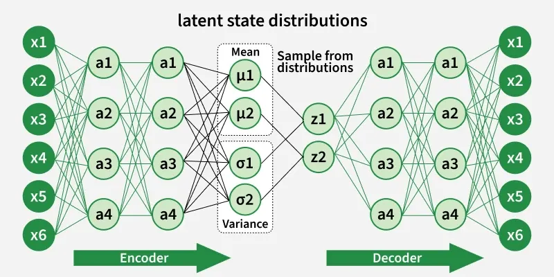
Variational Autoencoder
VAE is a special kind of autoencoder that can generate new data instead of just compressing and reconstructing it. It has three main parts:
**1. Encoder (Understanding the Input)
The encoder takes input data like images or text and learns its key features. Instead of outputting one fixed value, it produces two vectors for each feature:
- **Mean (μ): A central value representing the data.
- **Standard Deviation (σ): It is a measure of how much the values can vary.
These two values define a range of possibilities instead of a single number.
**2. Latent Space (Adding Some Randomness)
Instead of encoding the input as one fixed point it pick a random point within the range given by the mean and standard deviation. This randomness lets the model create slightly different versions of data which is useful for generating new, realistic samples.
**3. Decoder (Reconstructing or Creating New Data)
The decoder takes the random sample from the latent space and tries to reconstruct the original input. Since the encoder gives a range, the decoder can produce new data that is similar but not identical to what it has seen.
**Mathematics behind Variational Autoencoder
Variational autoencoder uses KL-divergence as its loss function the goal of this is to minimize the difference between a supposed distribution and original distribution of dataset.
Suppose we have a distribution z and we want to generate the observation x from it. In other words we want to calculate p\left( {z|x} \right) We can do it by following way:
p\left( {z|x} \right) = \frac{{p\left( {x|z} \right)p\left( z \right)}}{{p\left( x \right)}}
But, the calculation of p(x) can be difficult:
p\left( x \right) = \int {p\left( {x|z} \right)p\left(z\right)dz}
This usually makes it an intractable distribution. Hence we need to approximate p(z|x) to q(z|x) to make it a tractable distribution. To better approximate p(z|x) to q(z|x) we will minimize the KL-divergence loss which calculates how similar two distributions are:
\min KL\left( {q\left( {z|x} \right)||p\left( {z|x} \right)} \right)
By simplifying the above minimization problem is equivalent to the following maximization problem :
{E_{q\left( {z|x} \right)}}\log p\left( {x|z} \right) - KL\left( {q\left( {z|x} \right)||p\left( z \right)} \right)
The first term represents the reconstruction likelihood and the other term ensures that our learned distribution q is similar to the true prior distribution p. Thus our total loss consists of two terms one is reconstruction error and other is KL divergence loss:
Loss = L\left( {x, \hat x} \right) + \sum\limits_j {KL\left( {{q_j}\left( {z|x} \right)||p\left( z \right)} \right)}
Implementing Variational Autoencoder
We will build a Variational Autoencoder using TensorFlow and Keras. The model will be trained on the Fashion-MNIST dataset which contains 28×28 grayscale images of clothing items. This dataset is available directly through Keras.
Step 1: Importing Libraries
First we will be importing Numpy, TensorFlow, Keras layers and Matplotlib for this implementation.
python `
import numpy as np import tensorflow as tf import keras from keras import layers
`
Step 2: Creating a Sampling Layer
The sampling layer acts as the bottleneck, taking the mean and standard deviation from the encoder and sampling latent vectors by adding randomness. This allows the VAE to generate varied outputs.
- **epsilon = tf.random.normal(shape=tf.shape(mean)): Generate random noise from normal distribution.
- **return mean + tf.exp(0.5 * log_var) * epsilon: Apply reparameterization trick to sample latent vector. python `
class Sampling(layers.Layer): """Uses (mean, log_var) to sample z, the vector encoding a digit."""
def call(self, inputs):
    mean, log_var = inputs
    batch = tf.shape(mean)[0]
    dim = tf.shape(mean)[1]
    epsilon = tf.random.normal(shape=(batch, dim))
    return mean + tf.exp(0.5 * log_var) * epsilon
`
Step 3: Defining Encoder Block
The encoder takes input images and outputs two vectors: mean and log variance. These describe the distribution from which latent vectors are sampled.
- **x = layers.Dense(128, activation="relu")(x): Fully connected layer with 128 units and ReLU activation.
- **encoder = keras.Model(encoder_inputs, [mean, log_var, z], name="encoder"): Define encoder model from input to outputs. Python `
latent_dim = 2
encoder_inputs = keras.Input(shape=(28, 28, 1)) x = layers.Conv2D(64, 3, activation="relu", strides=2, padding="same")(encoder_inputs) x = layers.Conv2D(128, 3, activation="relu", strides=2, padding="same")(x) x = layers.Flatten()(x) x = layers.Dense(16, activation="relu")(x) mean = layers.Dense(latent_dim, name="mean")(x) log_var = layers.Dense(latent_dim, name="log_var")(x) z = Sampling()([mean, log_var]) encoder = keras.Model(encoder_inputs, [mean, log_var, z], name="encoder") encoder.summary()
`
**Output:

Summary
Step 4: Defining Decoder Block
Now we will define the architecture of decoder part of our autoencoder which takes sampled latent vectors and reconstructs the image.
- **x = layers.Dense(128, activation="relu")(latent_inputs): Dense layer to expand latent vector.
- **x = layers.Dense(28 * 28, activation="sigmoid")(x): Output layer to generate 784 pixels with values between 0 and 1. python `
latent_inputs = keras.Input(shape=(latent_dim,)) x = layers.Dense(7 * 7 * 64, activation="relu")(latent_inputs) x = layers.Reshape((7, 7, 64))(x) x = layers.Conv2DTranspose(128, 3, activation="relu", strides=2, padding="same")(x) x = layers.Conv2DTranspose(64, 3, activation="relu", strides=2, padding="same")(x) decoder_outputs = layers.Conv2DTranspose( 1, 3, activation="sigmoid", padding="same")(x) decoder = keras.Model(latent_inputs, decoder_outputs, name="decoder") decoder.summary()
`
**Output:

Summary
Step 5: Defining the VAE Model
Combine encoder and decoder into the VAE model and define the custom training step including reconstruction and KL-divergence losses.
- **self.loss_fn = keras.losses.BinaryCrossentropy(from_logits=False): Set reconstruction loss as binary cross-entropy.
- **with tf.GradientTape() as tape: Record operations for gradient calculation.
- **kl_loss = -0.5 * tf.reduce_mean(1 + log_var - tf.square(mean) - tf.exp(log_var)): Calculate KL divergence loss. python `
class VAE(keras.Model): def init(self, encoder, decoder, **kwargs): super().init(**kwargs) self.encoder = encoder self.decoder = decoder self.total_loss_tracker = keras.metrics.Mean(name="total_loss") self.reconstruction_loss_tracker = keras.metrics.Mean( name="reconstruction_loss" ) self.kl_loss_tracker = keras.metrics.Mean(name="kl_loss")
@property
def metrics(self):
    return [
        self.total_loss_tracker,
        self.reconstruction_loss_tracker,
        self.kl_loss_tracker,
    ]

def train_step(self, data):
    with tf.GradientTape() as tape:
        mean, log_var, z = self.encoder(data)
        reconstruction = self.decoder(z)
        reconstruction_loss = tf.reduce_mean(
            tf.reduce_sum(
                keras.losses.binary_crossentropy(data, reconstruction),
                axis=(1, 2),
            )
        )
        kl_loss = -0.5 * (1 + log_var - tf.square(mean) - tf.exp(log_var))
        kl_loss = tf.reduce_mean(tf.reduce_sum(kl_loss, axis=1))
        total_loss = reconstruction_loss + kl_loss
    grads = tape.gradient(total_loss, self.trainable_weights)
    self.optimizer.apply_gradients(zip(grads, self.trainable_weights))
    self.total_loss_tracker.update_state(total_loss)
    self.reconstruction_loss_tracker.update_state(reconstruction_loss)
    self.kl_loss_tracker.update_state(kl_loss)
    return {
        "loss": self.total_loss_tracker.result(),
        "reconstruction_loss": self.reconstruction_loss_tracker.result(),
        "kl_loss": self.kl_loss_tracker.result(),
    }
`
Step 6: Training the VAE
Load the Fashion-MNIST dataset and train the model for 10 epochs.
- **x_train = np.expand_dims(x_train, -1): Add channel dimension to training images.
- **x_test = x_test.astype("float32") / 255.0: Normalize test images.
- **x_test = np.expand_dims(x_test, -1): Add channel dimension to test images. python `
(x_train, _), (x_test, _) = keras.datasets.fashion_mnist.load_data() fashion_mnist = np.concatenate([x_train, x_test], axis=0) fashion_mnist = np.expand_dims(fashion_mnist, -1).astype("float32") / 255
vae = VAE(encoder, decoder) vae.compile(optimizer=keras.optimizers.Adam()) vae.fit(fashion_mnist, epochs=10, batch_size=128)
`
**Output:

Training
Step 7: Displaying Sampled Images
Generate new images by sampling points from the latent space and display them.
- **z_sample = np.array([[xi, yi]]): Create latent vector from grid point.
- **x_decoded = decoder.predict(z_sample): Decode latent vector to image. python `
import matplotlib.pyplot as plt
def plot_latent_space(vae, n=10, figsize=5):
img_size = 28
scale = 0.5
figure = np.zeros((img_size * n, img_size * n))

grid_x = np.linspace(-scale, scale, n)
grid_y = np.linspace(-scale, scale, n)[::-1]

for i, yi in enumerate(grid_y):
    for j, xi in enumerate(grid_x):
        sample = np.array([[xi, yi]])
        x_decoded = vae.decoder.predict(sample, verbose=0)
        images = x_decoded[0].reshape(img_size, img_size)
        figure[
            i * img_size : (i + 1) * img_size,
            j * img_size : (j + 1) * img_size,
        ] = images

plt.figure(figsize=(figsize, figsize))
start_range = img_size // 2
end_range = n * img_size + start_range
pixel_range = np.arange(start_range, end_range, img_size)
sample_range_x = np.round(grid_x, 1)
sample_range_y = np.round(grid_y, 1)
plt.xticks(pixel_range, sample_range_x)
plt.yticks(pixel_range, sample_range_y)
plt.xlabel("z[0]")
plt.ylabel("z[1]")
plt.imshow(figure, cmap="Greys_r")
plt.show()
plot_latent_space(vae)
`
**Output:

Sampled Images
Step 8: Displaying Latent Space Clusters
Encode the test set images and plot their positions in latent space to visualize clusters.
- **mean, _, _ = encoder.predict(x_test): Encode test images to latent mean vectors. python `
def plot_label_clusters(encoder, decoder, data, test_lab): z_mean, _, _ = encoder.predict(data) plt.figure(figsize=(12, 10)) sc = plt.scatter(z_mean[:, 0], z_mean[:, 1], c=test_lab) cbar = plt.colorbar(sc, ticks=range(10)) cbar.ax.set_yticklabels([labels.get(i) for i in range(10)]) plt.xlabel("z[0]") plt.ylabel("z[1]") plt.show()
labels = {0: "T-shirt / top", 1: "Trouser", 2: "Pullover", 3: "Dress", 4: "Coat", 5: "Sandal", 6: "Shirt", 7: "Sneaker", 8: "Bag", 9: "Ankle boot"}
(x_train, y_train), _ = keras.datasets.fashion_mnist.load_data() x_train = np.expand_dims(x_train, -1).astype("float32") / 255 plot_label_clusters(encoder, decoder, x_train, y_train)
`
**Output:

Latent Space Clusters
We can see that our model is working fine.
You can download source code from here.