Markov Decision Process (MDP) in Reinforcement Learning (original) (raw)
Last Updated : 4 Feb, 2026
Markov Decision Process (MDP) is a mathematical framework that models sequential decision-making using states, actions, rewards and transitions. In Reinforcement Learning, MDP provides the formal structure that defines the environment and guides how decisions are evaluated over time.
- An MDP consists of an agent that interacts with an environment over a sequence of time steps.
- At each step, the agent observes the current state, selects an action, and receives a reward from the environment.
- The environment then transitions to a new state based on the chosen action, following the Markov property.
- This structured formulation allows Reinforcement Learning algorithms to learn optimal policies that maximise long-term rewards.
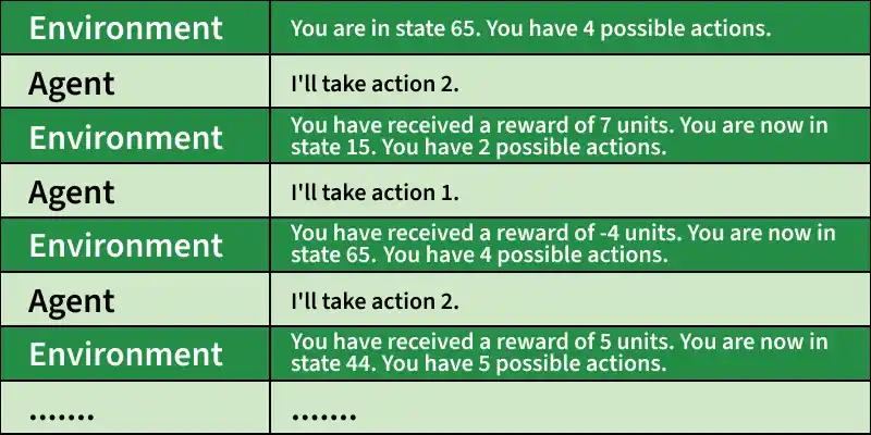
Agent–Environment Interaction in Reinforcement Learning
Components of MDP
- **Agent: The decision-maker that learns by interacting with the environment to achieve a goal.
- **Environment: Everything the agent interacts with, which responds to the agent’s actions by changing states and giving rewards.
- **State (S): A representation of the current situation of the environment at a given time.
- **Action (A): A choice made by the agent that influences the next state of the environment.
- **Reward (R): A numerical feedback signal that evaluates the quality of an action taken by the agent.
Understanding a MDP in Reinforcement Learning
A Markov Decision Process (MDP) provides a formal framework to model sequential decision-making in Reinforcement Learning. It defines how an agent interacts with an environment through states, actions and rewards to learn optimal behavior over time.
1. States
States describe the current situation of the environment and contain all information relevant for decision making.
S = \{ s_1, s_2, \ldots, s_N \}, \quad |S| = N
Here, S denotes the finite set of all possible states and N is the total number of states.
2. Actions
Actions represent the possible decisions an agent can take to influence the state of the environment.
A = \{ a_1, a_2, \ldots, a_K \}, \quad |A| = K
Here, A denotes the finite set of all possible actions and K is the total number of actions. For a given state s \in S, the set of allowable actions is denoted by A(s), where A(s) \subseteq A.
3. Transition Function
The transition function defines how the environment changes state when an action is taken, capturing the uncertainty in action outcomes. The process is Markovian, meaning the next state depends only on the current state and action, not on past history.
P(s_{t+1} \mid s_t, a_t) = T(s_t, a_t, s_{t+1})
Here T(s_t, a_t, s_{t+1}) represents the probability of moving to state s_{t+1} after taking action in state s_{t} .
This property ensures that the current state contains all information needed for optimal decision making.
4. Reward Function
The reward function provides a numerical feedback signal that guides the agent toward achieving its goal.
R : S \times A \times S \rightarrow \mathbb{R}
Here R(s,a,s') denotes the reward received when the agent takes action a in state s and transitions to state s'.
The reward function implicitly defines the learning objective by assigning positive, negative or zero values to outcomes, encouraging desirable behavior and discouraging undesirable actions.
5. Markov Decision Process (MDP)
A Markov Decision Process combines states, actions, transition dynamics and rewards into a single mathematical model for sequential decision making.
MDP=<S,A,T,R>
This framework can represent both episodic tasks (with terminal or absorbing states) and continuing tasks within the same model.
6. Policies
A policy defines the strategy an agent follows to choose actions in different states of an MDP, guiding its behavior while interacting with the environment.
**1. Deterministic policy: A deterministic policy always selects the same action in a given state
\pi : S \rightarrow A
**2. Stochastic Policy: A stochastic policy assigns probabilities to possible actions
\pi : S \times A \rightarrow [0,1], \quad \sum_{a \in A} \pi(s,a) = 1
By following a policy, the agent generates a sequence of states, actions and rewards, thereby controlling the environment modeled as an MDP.
7. Optimality Criteria and Discounting
Here we defines what it means for an agent to behave optimally in an MDP by specifying how rewards over time should be evaluated.
**1. Finite horizon: Optimizes the total expected reward over a fixed number of future steps.
\mathbb{E}\!\left[ \sum_{t=0}^{h} r_t \right]
Here we sums rewards from the current step up to a predefined horizon h.
**2. Discounted infinite horizon: Maximizes cumulative reward over an unlimited time while giving less weight to distant future rewards.
\mathbb{E}\!\left[ \sum_{t=0}^{\infty} \gamma^{t} r_t \right], \quad 0 \le \gamma < 1
Here, the discount factor \gamma reduces the influence of rewards received further in the future.
**3. Average reward: Focuses on maximizing the long-term average reward per time step.
\lim_{h \to \infty} \mathbb{E}\!\left[ \sum_{t=0}^{h} r_t \right]
This expression computes the expected reward per step as time progresses to infinity.
Value Functions
Value functions measure how good it is for an agent to be in a state or take an action, helping Reinforcement Learning agents learn optimal policies.
1. State Value Function
The state value function represents the expected cumulative reward for starting in a state s and following a policy \pi.
V^{\pi}(s) = \mathbb{E}_\pi \Bigg[ \sum_{t=0}^{\infty} \gamma^t R(s_t, a_t, s_{t+1}) \,\Big|\, s_0 = s \Bigg]
It calculates the total expected reward from state s, considering future rewards discounted by \gamma.
2. Action Value Function
The action value function evaluates the expected reward of taking a specific action a in state s and then following policy \pi.
Q^\pi(s,a) = \mathbb{E}_\pi \Big[ R(s,a,s') + \gamma V^\pi(s') \Big]
It combines the immediate reward for action a with the discounted value of the next state.
3. Bellman Equations
Value functions are recursive:the value of a state equals the immediate reward plus the discounted value of future states. This principle allows learning algorithms to update values iteratively without needing to simulate all future steps.
**State value function:
V^{\pi}(s) = \sum_{s'} P(s' \mid s, \pi(s)) \Big[ R(s, \pi(s), s') + \gamma V^{\pi}(s') \Big]
**Action value function:
Q^{\pi}(s,a) = \sum_{s'} P(s' \mid s, a) \Big[ R(s, a, s') + \gamma Q^{\pi}(s', \pi(s')) \Big]
These equations express that the value of a state or action equals the immediate reward plus the discounted value of future states.
4. Optimal Value Functions and Policy
Optimal value functions represent the maximum achievable reward, and the optimal policy selects actions that achieve it.
\begin{aligned}V^*(s) &= \max_a Q^*(s,a), \\Q^*(s,a) &= \sum_{s'} P(s' \mid s,a) \Big[ R(s,a,s') + \gamma \max_{a'} Q^*(s',a') \Big]\end{aligned}
The optimal state value is the best possible return from a state, and the optimal action chooses the action with the highest expected reward.
MDP in Reinforcement Learning using Grid Game
Here we shows a grid-based game to demonstrate how an agent navigates an environment using MDP, making decisions to maximize rewards while avoiding penalties.
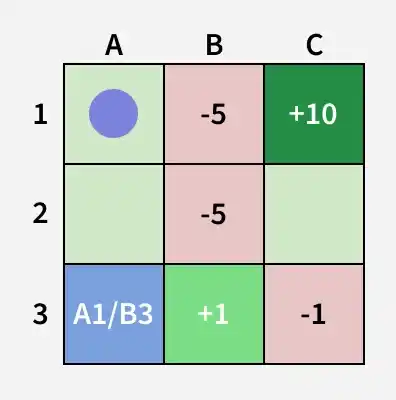
Enviroment
**Q-learning: Markov Decision Process + Reinforcement Learning
**Step 1: In Q-learning, the agent learns optimal actions by interacting with the environment without knowing transition probabilities in advance, making it useful when probabilities and rewards are unknown.
**Step 2: The agent updates a Q-table of state-action pairs, where each cell stores the expected value of taking an action in a state, starting from 0 and refined iteratively using the Bellman Equation.
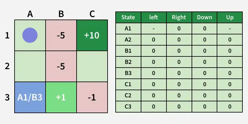
Q-table
**Step 3: The agent updates the Q-table based on actions taken, learning from penalties and rewards; for example, moving right may incur -5, while moving down may have a higher expected value.
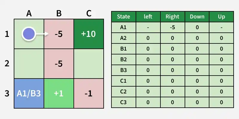
Update Q-table
**Step 4: The agent moves along a path, updates the Q-table with rewards received (e.g., reaching C1 gives +10), but initial Q-values are incomplete and refined over multiple iterations.

Goal State
**Step 5: Q-values are updated using the Bellman Equation, with recent information sometimes weighted more than older values using a discount factor gamma.
**Step 6: The agent balances exploration and exploitation, trying new paths while leveraging known high-value actions, gradually converging on an optimal policy over multiple iterations.
Solving MDPs in Reinforcement Learning
Several algorithms have been developed to solve MDPs within the RL framework. Here are a few key approaches:
1. Dynamic Programming
Dynamic programming methods, such as Value Iteration and Policy Iteration, are used to solve MDPs when the model of the environment (transition probabilities and rewards) is known.
- **Value Iteration: Iteratively updates the value function until it converges to the optimal value function.
V_{k+1}(s) = \max_{a \epsilon A} P(s'|s,a) [R(s,a,s')+ \gamma V_k (s')]
- **Policy Iteration: Alternates between policy evaluation and policy improvement until the policy converges to the optimal policy.
2. Monte Carlo Methods
Monte Carlo methods are used when the model of the environment is unknown. These methods rely on sampling to estimate value functions and optimize policies.
- **First-Visit MC: Estimates the value of a state as the average return following the first visit to that state.
- **Every-Visit MC: Estimates the value of a state as the average return following all visits to that state.
3. Temporal-Difference Learning
Temporal-Difference (TD) learning methods combine ideas from dynamic programming and Monte Carlo methods. TD learning updates value estimates based on the difference (temporal difference) between consecutive value estimates.
- **SARSA (State-Action-Reward-State-Action): Updates the action-value function based on the action taken by the current policy.
Q(s_t,a_t)←Q(s_t,a_t)+α[R_{t+1}+γQ(s_{t+1},a_{t+1} )−Q(s_t,a_t )]
- **Q-Learning: An off-policy TD control algorithm that updates the action-value function based on the maximum reward of the next state.
Q(s_t, a_t) ← Q(s_t, a_t) + \alpha [R_{t+1} + \gamma \max_a Q(s_{t+1}, a) - Q(s_t, a_t)]
Markov Decision Processes (MDPs) provide a formal framework for modeling decision-making in uncertain environments. They form the theoretical foundation of Reinforcement Learning, enabling the development of effective RL solutions.