What is Perceptron (original) (raw)
Last Updated : 9 May, 2026
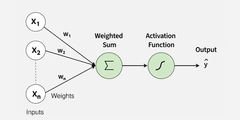
A Perceptron is the simplest form of a neural network that makes decisions by combining inputs with weights and applying an activation function. It is mainly used for binary classification problems. It forms the basic building block of many deep learning models.
- Takes multiple inputs and assigns weights
- Computes a weighted sum and applies a threshold
- Outputs either 0 or 1 (binary outcome)
- Forms the foundation of larger neural networks
Core Components
Perceptron
1. Inputs (x_1,x_2,...,x_n)
These are the features or measurable attributes of a data point that the perceptron uses to make a decision. Each input provides a signal that contributes to the final output.
- **Example: For an OR gate, the inputs are binary: (x_1, x_2) \in \{0,1\}^2
- Inputs themselves have no inherent influence unless multiplied by weights.
2. Weights (w_1,w_2,...,w_n)
Weights determine how strongly each input contributes to the prediction. A larger weight means the corresponding input has a higher impact.
- Weights are learned during training, adjusting based on errors.
- They act like importance scores for each feature.
3. Bias (b)
The bias is a constant value added to the weighted sum to shift the decision boundary.
- It allows the perceptron to classify correctly even when all input features are zero.
- Bias ensures the model is not forced to pass the decision boundary through the origin.
Difference Between Weights and Bias
- Weights control how much each input influences the output.
- Bias controls when the perceptron activates, independent of any input.
- Mathematically, Weights tilt the line and Bias shifts the line up/down or left/right.
4. Net Input (Weighted Sum)
This is the combined effect of all inputs and their weights:
z = \sum_{i=1}^{n} w_i x_i + b
- Represents the activation strength before passing through the activation function.
- If z is high or low enough, it determines the final class.
5. Activation Function (Step Function)
The activation function converts the numerical input into a binary output:
\hat{y} =\begin{cases}1 & \text{if } z \ge 0 \\0 & \text{otherwise}\end{cases}
- It introduces non-linearity in the decision-making, although the decision boundary remains linear.
- Output is always 0 or 1 making perceptrons suitable for binary classification.
Fundamentals of Neural Network
A neural network extends the perceptron by connecting many neurons across multiple layers.
**1. Input layer: The input layer provides the network with the raw feature vector:
x=(x_1,x_2,...,x_n)
- No computation happens here.
- It simply passes the input values to the next layer.
**2. Hidden layers: Hidden layers contain multiple perceptrons (neurons) that learn intermediate representations of the data.
**Hidden Layer Computation:
z^{(1)}=W^{(1)}\mathbf{x}+b^{(1)}
a^{(1)}=\sigma(z^{(1)})
**where:
- W^{(1)}: weight matrix for hidden layer
- b^{(1)}: bias vector
- \sigma: non-linear activation function (ReLU, Sigmoid, Tanh, etc.)
- Hidden layers identify complex patterns not visible from raw input alone.
- Adding more hidden layers improves model expressiveness.
**3. Output layer: The output layer produces the final prediction, which may be binary, multi-class or a continuous value.
**Output Layer Computation:
z^{(2)}=W^{(2)}a^{(1)}+b^{(2)}
\hat{y} = \sigma (z^{(2)})
Output activation depends on the task:
- **Sigmoid: binary classification
- **Softmax: multi-class classification
- **Linear: regression
Because of multiple layers and non-linear activations, neural networks can model complex, non-linear decision boundaries, while a single perceptron can only model a straight line.
Working
Training a perceptron means finding suitable weights wi and bias b such that most training points are correctly classified.
1. Compute the Weighted Sum
The perceptron first calculates a weighted combination of the input features, along with a bias term that helps shift the decision boundary.
z = \sum_{i=1}^{n} w_i x_i + b
2. Apply the Activation Function (Step Function)
The perceptron uses a simple threshold activation to convert the numerical value into a binary class label.
\hat{y} =\begin{cases}1 & \text{if } z \ge 0 \\0 & \text{otherwise}\end{cases}
3. Compare Prediction with Actual Output
The perceptron checks if the predicted output matches the true label.
\text{error} = y - \hat{y}
4. Update the Weights (Learning Rule)
Whenever the perceptron misclassifies a sample, it updates each weight by an amount proportional to the error and the input value.
w_i \leftarrow w_i + \eta (y - \hat{y}) x_i
5. Update the Bias Term
The bias is adjusted similarly to shift the decision boundary left or right.
b \leftarrow b + \eta (y - \hat{y})
6. Repeat for All Samples Across Multiple Epochs
The perceptron cycles through the entire dataset several times (epochs), refining weights gradually until it reaches a stable solution.
7. Final Learned Model
After training, the perceptron produces predictions using:
\hat{y} = \text{step}(\mathbf{w}^\top \mathbf{x} + b)
Implementation
Let's implement the model:
Step 1: Import Libraries and Create the Dataset
We import NumPy for numerical operations and Matplotlib for visualizations. The dataset represents the OR logic gate, which is linearly separable and suitable for perceptron learning.
Python `
import numpy as np import matplotlib.pyplot as plt
X_or = np.array([ [0, 0], [0, 1], [1, 0], [1, 1] ])
y_or = np.array([0, 1, 1, 1])
`
Step 2: Define the Perceptron Class
This defines the entire Perceptron class: constructor, predict and .fit() trains the model by adjusting weights and bias whenever a misclassification occurs and tracks errors per epoch.
Python `
class Perceptron: def init(self, learning_rate=0.1, epochs=20): self.lr = learning_rate self.epochs = epochs self.weights = None self.bias = None self.errors_per_epoch = [] def predict(self, X): linear_output = np.dot(X, self.weights) + self.bias return np.where(linear_output >= 0, 1, 0) def fit(self, X, y): n_samples, n_features = X.shape self.weights = np.zeros(n_features) self.bias = 0.0 for _ in range(self.epochs): errors = 0 for xi, target in zip(X, y): linear_output = np.dot(xi, self.weights) + self.bias y_pred = 1 if linear_output >= 0 else 0 update = self.lr * (target - y_pred) self.weights += update * xi self.bias += update errors += int(update != 0) self.errors_per_epoch.append(errors)
`
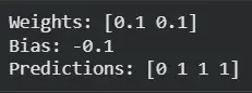
Step 3: Train the Perceptron on OR Data
- We create a perceptron instance and train it on the OR dataset.
- After training, we print the learned weights, bias and predictions (which should be [0 1 1 1] for the OR gate). Python `
p_or = Perceptron(learning_rate=0.1, epochs=20) p_or.fit(X_or, y_or)
print("Weights:", p_or.weights) print("Bias:", p_or.bias) print("Predictions:", p_or.predict(X_or))
`
**Output:
Result
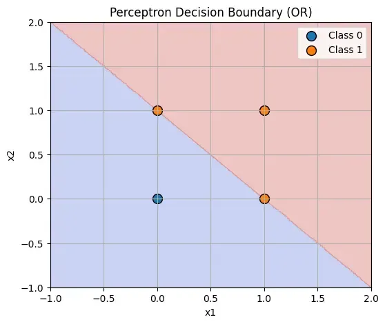
Step 4: Decision Boundary Plot
- We build a dense grid over the input space, predict the class at each grid point and color the regions.
- Then we overlay the real OR data points to show how the perceptron separates class 0 and class 1. Python `
def plot_decision_boundary(X, y, model, title): x_min, x_max = X[:, 0].min() - 1, X[:, 0].max() + 1 y_min, y_max = X[:, 1].min() - 1, X[:, 1].max() + 1
xx, yy = np.meshgrid(
    np.linspace(x_min, x_max, 300),
    np.linspace(y_min, y_max, 300)
)

grid = np.c_[xx.ravel(), yy.ravel()]
Z = model.predict(grid)
Z = Z.reshape(xx.shape)

plt.figure(figsize=(6, 5))
plt.contourf(xx, yy, Z, alpha=0.3, cmap="coolwarm")

for label in np.unique(y):
    pts = X[y == label]
    plt.scatter(pts[:, 0], pts[:, 1],
                s=100, edgecolor='black',
                label=f"Class {label}")

plt.title(title)
plt.xlabel("x1")
plt.ylabel("x2")
plt.legend()
plt.grid(True)
plt.show()
plot_decision_boundary(X_or, y_or, p_or, "Perceptron Decision Boundary (OR)")
`
**Output:
Plot
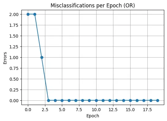
Step 5: Plot Misclassifications per Epoch
- This graph shows how the training error changes over epochs.
- For a linearly separable problem like OR, the misclassifications should quickly drop to zero, indicating convergence. Python `
plt.figure(figsize=(6, 4)) plt.plot(p_or.errors_per_epoch, marker='o') plt.title("Misclassifications per Epoch (OR)") plt.xlabel("Epoch") plt.ylabel("Errors") plt.grid(True) plt.show()
`
**Output:
Plot
Perceptron vs. Multi-Layer Perceptron (MLP)
Lets compare perceptron and multi-layer perceptron,
| **Aspect | **Perceptron | **Multi-Layer Perceptron (MLP) |
|---|---|---|
| **Model Depth | Single layer with no hidden neurons. | Multiple layers with one or more hidden layers. |
| **Type of Patterns Learned | Learns only linear relationships; straight-line separation. | Learns complex, non-linear patterns and curved boundaries. |
| **Problem-Solving Ability | Cannot solve XOR or non-linearly separable problems. | Easily solves XOR and other complex classification tasks. |
| **Activation Functions | Uses a simple step function (hard 0/1 output). | Uses advanced activations like ReLU, Sigmoid, Tanh for richer learning. |
| **Learning Method | Trained with a simple perceptron update rule. | Trained using backpropagation and gradient descent. |
| **Real-World Use | Limited to simple demonstrations and basic classification. | Used in real-world AI systems like vision, NLP and deep learning applications. |
Applications
- **Binary Classification: Used for simple yes/no decision problems such as spam detection or basic quality checks.
- **Logic Gate Modelling: Implements linearly separable gates like AND or NAND with perfect accuracy.
- **Pattern Recognition Basics: Helps identify simple patterns where classes can be separated with a straight line.
- **Feature Importance Insight: Weight values indicate which features influence the output more strongly.
- **Educational Tool: Commonly used to teach foundations of machine learning and neural networks.
Advantages
- **Simple Architecture: Easy to understand, implement and visualize as a basic neural model.
- **Fast Training: Lightweight computations make learning very quick even on small devices.
- **Works on Linearly Separable Data: Achieves perfect performance when a straight-line boundary exists.
- **Low Resource Requirement: Requires minimal memory and computation, suitable for tiny datasets.
- **Foundation for Deep Learning: Forms the conceptual basis for multilayer perceptrons and complex networks.
Limitations
- **No Non-Linear Learning: Fails on problems like XOR where a curved or complex boundary is needed.
- **Binary Output Only: Cannot handle multi-class or probabilistic outcomes without extensions.
- **No Hidden Layers: Lacks depth, making it unable to learn hierarchical or abstract patterns.
- **Sensitive to Data Scale: Performance drops if features are not normalized or scaled properly.
- **Not Suitable for Real-World ML: Too simplistic for modern tasks like vision, NLP or sequence modeling.