YOLO : You Only Look Once Real Time Object Detection (original) (raw)

Last Updated : 14 Nov, 2025

YOLO was proposed by Joseph Redmond _et al. in 2015 to deal with the problems faced by the object recognition models at that time, Fast R-CNN was one of the models at that time but it had its own challenges such as that network could not be used in real-time because it took 2-3 seconds to predict an image and therefore could not be used in real-time. Whereas in YOLO we have to look only once in the network i.e. only one forward pass is required through the network to make the final predictions.

**YOLO Architecture

YOLO

**1. Input Preprocessing:

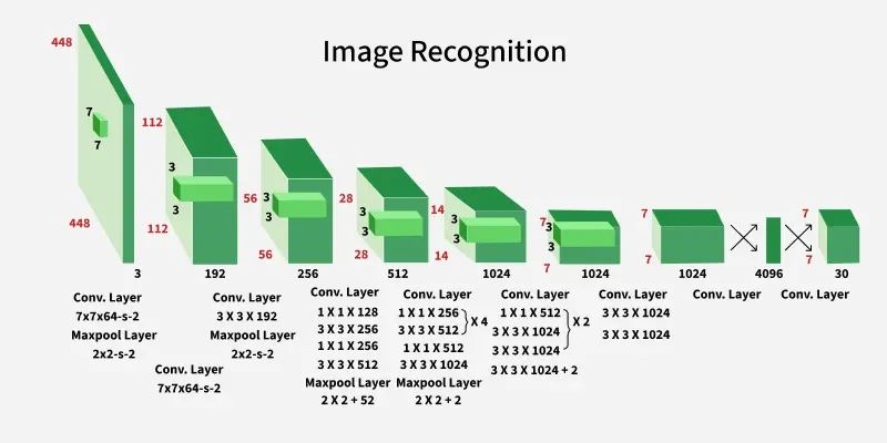
The model accepts an image as input. It resizes the input image to 448×448 pixels ensuring that the aspect ratio is preserved using padding. This ensures uniformity of input dimensions across the network which is essential for batch processing in deep learning.

**2. Backbone Convolutional Neural Network (CNN):

After preprocessing the image is passed through a deep CNN architecture designed for object detection:

• The model consists of **24 convolutional layers and **4 max-pooling layers.
• These layers help in extracting hierarchical spatial features from the image.

**3. Use of 1×1 and 3×3 Convolutions:

• To reduce the number of parameters and compress channels, 1×1 convolutions are employed.
• These are followed by 3×3 convolutions to capture spatial patterns in the feature maps.

This design pattern i.e 1×1 followed by 3×3 improves computational efficiency while maintaining expressive power.

**4. Fully Connected Layers:

Following the convolutional layers, the architecture has 2 fully connected layers. The final fully connected layer produces an output of shape (1, 1470).

**5. Cuboidal Prediction Output:

The output vector of size 1470 is reshaped to (7, 7, 30). Here, 7×7 represents the grid cells, and 30 represents the prediction vector for each cell:

30 = (2 \text{ bounding boxes} \times 5) + (20 \text{ class probabilities})

**6. Activation Functions:

The architecture predominantly uses Leaky ReLU as its activation function. The Leaky ReLU is defined as:

f(x) = \begin{cases} x, & \text{if } x > 0 \\ 0.01x, & \text{if } x \leq 0 \end{cases}

This activation allows a small gradient when the unit is not active, preventing dead neurons.

**7. Output Layer Activation:

The last layer uses a linear activation function, suitable for making raw predictions like bounding box coordinates and confidence scores.

**8. Regularization Techniques:

1. **Batch Normalization is employed across layers to stabilize and accelerate training.
2. **Dropout is also incorporated to prevent overfitting by randomly deactivating neurons during training, encouraging the network to learn more robust features.

**Training Process

• This model is trained on the ImageNet-1000 dataset. The model is trained over a week and achieve top-5 accuracy of 88% on ImageNet 2012 validation which is comparable to GoogLeNet (2014 ILSVRC winner).
• Fast YOLO uses fewer layers (9 instead of 24) and fewer filters. Except this, the fast YOLO have all parameters similar to YOLO.
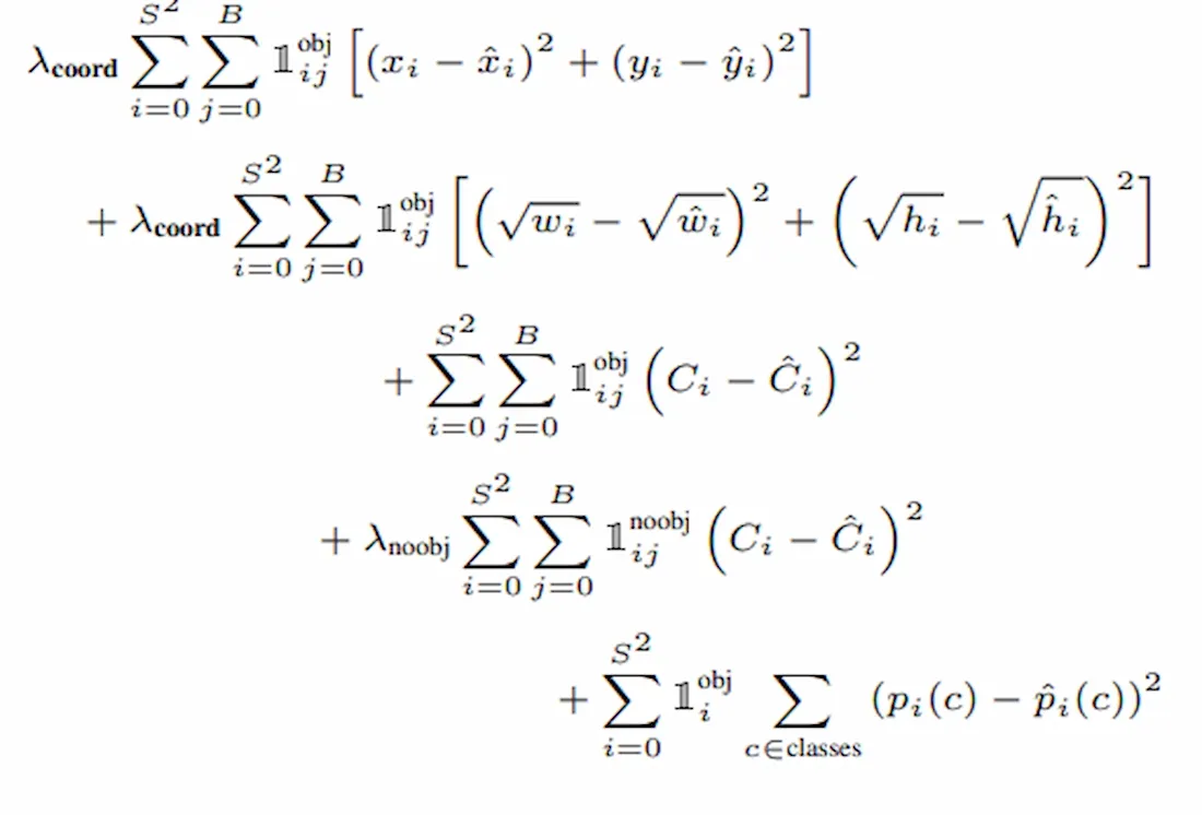
• YOLO uses sum-squared error loss function which is easy to optimize. However, this function gives equal weight to the classification and localization task. The loss function defined in YOLO as follows:

Formula

where,

• l_{i}^{obj} denotes if object is present in cell _i.
• l_{ij}^{obj} denotes j_{th} bounding box responsible for prediction of object in the cell _i.
• \lambda_{coord} and \lambda_{noobj} are regularization parameter required to balance the loss function.

In this model, we take \lambda_{coord}=5 and \lambda_{noobj}=5.

The first two parts of the above loss equation represent localization mean-squared error, but the other three parts represent classification error.

Localization Error

1. The first term calculates the deviation from the ground truth bounding box.
2. The second term calculates the square root of the difference between height and width of the bounding box. In the second term, we take the square root of width and height because our loss function should be able to consider the deviation in terms of the size of the bounding box.
3. For small bounding boxes, the little deviation should be more important as compared to large bounding boxes.

Classification Loss

There are three terms in classification loss:

• The first term calculates the sum-squared error between the predicted confidence score that whether the object present or not and the ground truth for each bounding box in each cell.
• Similarly, the second term calculates the mean-squared sum of cells that do not contain any bounding box and a regularization parameter is used to make this loss small.
• The third term calculates the sum-squared error of the classes belongs to these grid cells.

**Detection

• This architecture divides the image into a grid of S*S size.
• If the centre of the bounding box of the object is in that grid, then this grid is responsible for detecting that object.
• Each grid predicts bounding boxes with their confidence score.
• Each confidence score shows how accurate it is that the bounding box predicted contains an object and how precise it predicts the bounding box coordinates with respect to ground truth prediction.

YOLO Image (divided into S*S grid)

At test time we multiply the conditional class probabilities and the individual box confidence predictions. We define our confidence score as follows :

\kern 6pc P_{r}\left( \text{Object} \right) * \text{IOU}_{\text{pred}}^{\text{truth}}

**Note: the confidence score should be 0 when there is no object exists in the grid. If there is an object present in the image the confidence score should be equal to IoU between ground truth and predicted boxes. Each bounding box consists of 5 predictions: (x, y, w, h) and confidence score. The (x, y) coordinates represent the centre of the box relative to the bounds of the grid cell. The h, w coordinates represents height, width of bounding box relative to (x, y). The confidence score represents the presence of an object in the bounding box.

YOLO single Grid Bounding box-Box

This results in combination of bounding boxes from each grid like this.

YOLO bounding box Combination

Each grid also predicts C conditional class probability, Pr (Classi | Object).

YOLO conditional probability map

This probability were conditional based on the presence of an object in grid cell. Regardless the number of boxes each grid cell predicts only one set of class probabilities. These prediction are encoded in the 3D tensor of size S * S * (5*B +C).

Now, we multiply the conditional class probabilities and the individual box confidence predictions,

YOLO output feature map

YOLO test Result

This gives us class-specific confidence scores for each box. These scores encode both the probability of that class appearing in the box and how well the predicted box fits the object. Then after we apply non-maximal suppression for suppressing the non max outputs (when a number of boxes are predicted for the same object). At last , our final predictions are generated.

YOLO is very fast at the test time because it uses only a single CNN architecture to predict results and class is defined in such a way that it treats classification as a regression problem.