Aggregate DemandAggregate Supply (ADAS) Approach (original) (raw)
Aggregate Demand-Aggregate Supply (AD-AS) Approach
Last Updated : 16 May, 2026
The Aggregate Demand–Aggregate Supply (AD–AS) approach is an important macroeconomic model used to explain the determination of national income, output, employment, and price level in an economy. It studies the interaction between total demand and total supply in the economy. Equilibrium is achieved where the Aggregate Demand (AD) curve intersects the Aggregate Supply (AS) curve.
The model helps explain economic problems such as inflation, unemployment, and business cycles.
Key Concepts
**Aggregate Demand (AD)
Aggregate Demand (AD) refers to the total demand for final goods and services in an economy at a given price level during a specific period.The AD curve slopes downward because a rise in the price level reduces purchasing power and demand.
The major components of Aggregate Demand are:
- **Consumption Expenditure (C): Spending by households on goods and services.
- **Investment Expenditure (I): Spending by firms on capital goods like machinery and buildings.
- **Government Expenditure (G): Expenditure by the government on infrastructure, public services, and welfare programs.
- **Net Exports (X – M): The difference between exports and imports of goods and services.
Hence, **Aggregate Demand (AD) = C + I + G + (X – M).
**Aggregate Supply (AS)
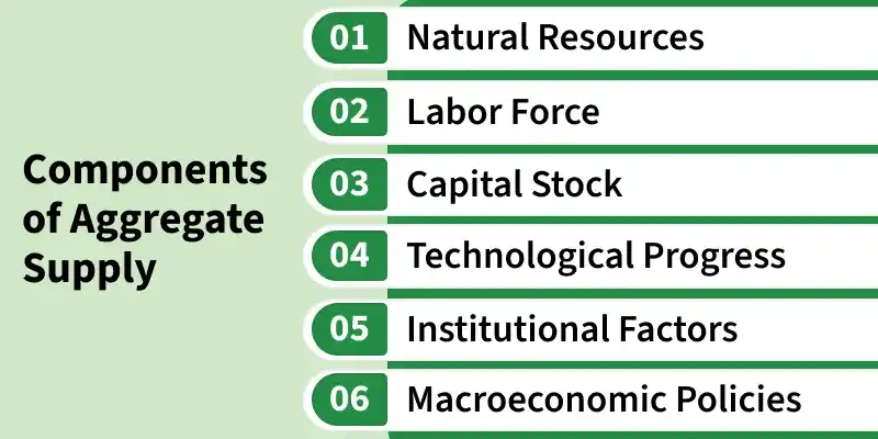
**Aggregate Supply (AS) refers to the total quantity of goods and services producers are willing to supply at a given price level.
Aggregate Supply is generally divided into two forms:
- **Short-Run Aggregate Supply (SRAS): It shows the relationship between output and price level when factor prices, such as wages, remain fixed. The SRAS curve slopes upward, indicating that producers increase output when prices rise.
- **Long-Run Aggregate Supply (LRAS): It represents the output level when all factors, including wages and resource prices, are fully flexible. The LRAS curve is vertical at the economy’s full-employment level of output, reflecting its maximum productive capacity.
**Assumptions
The determination of the equilibrium level of income and output under the AD–AS approach is based on certain assumptions. These assumptions simplify the analysis and help in understanding how aggregate demand and aggregate supply interact to determine macroeconomic equilibrium.
The main assumptions are as follows:
**Two-Sector Economy: The model considers only two sectors—households and firms. It assumes there is no role of government or foreign trade, meaning the economy is closed and includes only domestic production and consumption.
**Autonomous Investment: Investment expenditure is assumed to be autonomous, that is, independent of the level of income or output. This means that changes in national income do not influence the volume of investment in the short run.
**Constant Price Level: The general price level is assumed to remain constant. Prices and wages do not change in the short period, allowing the analysis to focus purely on real output and employment rather than inflation or deflation.
**Short-Run Period: The analysis is conducted for the short run, where productive capacity, technology, and factor availability remain fixed. Only output and employment levels adjust to changes in aggregate demand.
**Graphical Representation and Equilibrium
The equilibrium level of income and output in an economy is determined at the point where Aggregate Demand (AD) equals Aggregate Supply (AS). This is the point at which planned spending by households and firms matches the total output produced by the economy. At this level, there is no tendency for income or output to change, as the flow of goods and services is fully absorbed by aggregate expenditure.
In the AD–AS model:
- The AD curve slopes upward from left to right, showing that as income increases, total expenditure (C + I) also increases.
- The AS curve is a 45° line that represents all points where income equals output. It shows that whatever is produced in the economy is sold, ensuring equality between income and expenditure.
The equilibrium point is determined at the intersection of the AD and AS curves.

- At this point, planned savings equal planned investment, and the economy achieves a stable level of output and income.
- If AD is greater than AS, inventories fall, leading to an increase in production and income.
- If AD is less than AS, inventories accumulate, leading to a fall in production and income.
Thus, equilibrium is achieved where AD = AS, ensuring that the total spending equals total output in the economy.
**Determination of Equilibrium Level
According to Keynesian theory, the equilibrium level of income and output in an economy is determined where Aggregate Demand (AD) equals Aggregate Supply (AS). This represents the point at which planned total spending by households and firms matches the total value of goods and services produced in the economy.
In simple terms,
Equilibrium Condition****:** AD = AS
When this equality holds, the economy has no tendency to expand or contract output, as total demand exactly equals total supply.
- If AD > AS, total planned expenditure exceeds current output. Firms experience a fall in inventories and increase production, which raises income and output until equilibrium is restored.
- If AD < AS, total planned expenditure is less than total output. Firms face unplanned accumulation of inventories and reduce production, which lowers income and output until equilibrium is achieved.
The equilibrium ensures that all goods produced are sold and there is no unintended change in stock levels.
**Example Table
| Level of Income (₹ crore) | Aggregate Demand (₹ crore) | Aggregate Supply (₹ crore) | Situation in the Economy |
|---|---|---|---|
| 100 | 120 | 100 | AD > AS → Output increases |
| 200 | 200 | 200 | AD = AS → Equilibrium |
| 300 | 260 | 300 | AD < AS → Output decreases |
At income level ₹200 crore, AD equals AS, indicating the equilibrium level of income and output in the economy.
At this point, the level of aggregate demand that equals aggregate supply is known as Effective Demand, since it determines the actual level of income and employment in the economy.
**Short-Run Analysis
The Keynesian model primarily focuses on the short run, where prices are assumed to remain constant. In this period, output and employment are determined mainly by changes in aggregate demand rather than price movements.
In the short run:
- Firms can increase or decrease production to meet demand without altering prices.
- The level of employment and output depends on the volume of aggregate expenditure.
- The economy may operate below full employment, meaning resources are underutilized.
If aggregate demand increases, firms raise production to meet higher demand, leading to higher income and employment. Conversely, a fall in aggregate demand reduces output and employment, resulting in unemployment and lower income.
Thus, in the short-run analysis, output is demand-determined, and equilibrium is achieved where AD = AS at a fixed price level.
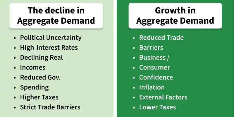
**Shifts in Aggregate Demand
In the short run, the equilibrium level of income and output in an economy can change when there is a shift in the Aggregate Demand (AD) curve. A shift occurs when any component of aggregate demand, such as consumption expenditure (C) or investment expenditure (I), changes due to factors other than income.
**Rightward Shift (Increase in AD)
When aggregate demand increases, the AD curve shifts rightward. This signifies that at the same price and income levels, people and firms are willing to purchase more goods and services. The main causes include:
- **Increase in Consumer Spending: When consumers become more confident about their future income or wealth, they tend to spend more on goods and services. This higher demand encourages firms to expand their production.
- **Higher Investment Expenditure: When business expectations are positive or when interest rates fall, firms invest more in capital goods to meet the expected rise in future demand.
As a result of these factors, firms experience greater demand for their products, leading to an increase in production, employment, and national income. The economy thus moves to a higher equilibrium level of income and output, represented by a new intersection point between AD and AS curves.
**Leftward Shift (Decrease in AD)
When aggregate demand decreases, the AD curve shifts leftward. This means that at the same income level, the total planned expenditure on goods and services falls. The main causes are:
- **Fall in Consumer Spending: When households expect a decline in income, or when prices rise, they reduce their consumption expenditure. This lowers the demand for goods and services.
- **Decrease in Investment Expenditure: When business expectations are pessimistic or when interest rates rise, firms cut back on investment spending, reducing overall demand in the economy.
Due to the fall in demand, firms face unsold inventories and are forced to reduce production. Consequently, employment and income levels decline, leading the economy to a lower equilibrium level of income and output.