Linear Regression in Machine learning (original) (raw)
Linear regression is a type of **supervised machine-learning algorithm that learns from the labelled datasets and maps the data points with most optimized linear functions which can be used for prediction on new datasets. It assumes that there is a linear relationship between the input and output, meaning the output changes at a constant rate as the input changes. This relationship is represented by a straight line.
**For example we want to predict a student's exam score based on how many hours they studied. We observe that as students study more hours, their scores go up. In the example of predicting exam scores based on hours studied. Here
- **Independent variable (input): Hours studied because it's the factor we control or observe.
- **Dependent variable (output): Exam score because it depends on how many hours were studied.
We use the independent variable to predict the dependent variable.
**Why Linear Regression is Important?
Here’s why linear regression is important:
- **Simplicity and Interpretability: It’s easy to understand and interpret, making it a starting point for learning about machine learning.
- **Predictive Ability: Helps predict future outcomes based on past data, making it useful in various fields like finance, healthcare and marketing.
- **Basis for Other Models: Many advanced algorithms, like logistic regression or neural networks, build on the concepts of linear regression.
- **Efficiency: It’s computationally efficient and works well for problems with a linear relationship.
- **Widely Used: It’s one of the most widely used techniques in both statistics and machine learning for regression tasks.
- **Analysis: It provides insights into relationships between variables (e.g., how much one variable influences another).
Best Fit Line in Linear Regression
In linear regression, the best-fit line is the straight line that most accurately represents the relationship between the independent variable (input) and the dependent variable (output). It is the line that minimizes the difference between the actual data points and the predicted values from the model.
1. Goal of the Best-Fit Line
The goal of linear regression is to find a straight line that minimizes the error (the difference) between the observed data points and the predicted values. This line helps us predict the dependent variable for new, unseen data.

Linear Regression
Here Y is called a dependent or target variable and X is called an independent variable also known as the predictor of Y. There are many types of functions or modules that can be used for regression. A linear function is the simplest type of function. Here, X may be a single feature or multiple features representing the problem.
2. Equation of the Best-Fit Line
For simple linear regression (with one independent variable), the best-fit line is represented by the equation
y = mx + b
**Where:
- **y is the predicted value (dependent variable)
- **x is the input (independent variable)
- **m is the slope of the line (how much y changes when x changes)
- **b is the intercept (the value of y when x = 0)
The best-fit line will be the one that optimizes the values of m (slope) and b (intercept) so that the predicted y values are as close as possible to the actual data points.
**3. Minimizing the Error: The Least Squares Method
To find the best-fit line, we use a method called **Least Squares. The idea behind this method is to minimize the sum of squared differences between the actual values (data points) and the predicted values from the line. These differences are called residuals.
The formula for residuals is:
Residual = yᵢ - ŷᵢ
**Where:
- yᵢ is the actual observed value
- ŷᵢ is the predicted value from the line for that xᵢ
The least squares method minimizes the sum of the squared residuals:
Sum of squared errors (SSE) = Σ(yᵢ - ŷᵢ)²
This method ensures that the line best represents the data where the sum of the squared differences between the predicted values and actual values is as small as possible.
**4. Interpretation of the Best-Fit Line
- **Slope (m): The slope of the best-fit line indicates how much the dependent variable (y) changes with each unit change in the independent variable (x). For example if the slope is 5, it means that for every 1-unit increase in x, the value of y increases by 5 units.
- **Intercept (b): The intercept represents the predicted value of y when x = 0. It’s the point where the line crosses the y-axis.
In linear regression some hypothesis are made to ensure reliability of the model's results.
Limitations
- **Assumes Linearity: The method assumes the relationship between the variables is linear. If the relationship is non-linear, linear regression might not work well.
- **Sensitivity to Outliers: Outliers can significantly affect the slope and intercept, skewing the best-fit line.
**Hypothesis function in Linear Regression
In linear regression, the hypothesis function is the equation used to make predictions about the dependent variable based on the independent variables. It represents the relationship between the input features and the target output.
For a simple case with one independent variable, the hypothesis function is:
h(x) = β₀ + β₁x
**Where:
- h(x) (or ŷ) is the predicted value of the dependent variable (y).
- x x is the independent variable.
- β₀ is the intercept, representing the value of y when x is 0.
- β₁ is the slope, indicating how much y changes for each unit change in x.
For **multiple linear regression (with more than one independent variable), the hypothesis function expands to:
h(x₁, x₂, ..., xₖ) = β₀ + β₁x₁ + β₂x₂ + ... + βₖxₖ
**Where:
- x₁, x₂, ..., xₖ are the independent variables.
- β₀ is the intercept.
- β₁, β₂, ..., βₖ are the coefficients, representing the influence of each respective independent variable on the predicted output.
**Assumptions of the Linear Regression
**1. Linearity: The relationship between inputs (X) and the output (Y) is a straight line.

Linearity
**2. Independence of Errors: The errors in predictions should not affect each other.
**3. Constant Variance (Homoscedasticity): The errors should have equal spread across all values of the input. If the spread changes (like fans out or shrinks), it's called heteroscedasticity and it's a problem for the model.

Homoscedasticity
**4. Normality of Errors: The errors should follow a normal (bell-shaped) distribution.
*5. No Multicollinearity _*(**_**for multiple regression): Input variables shouldn’t be too closely related to each other.
**6. No Autocorrelation: Errors shouldn't show repeating patterns, especially in time-based data.
**7. Additivity: The total effect on Y is just the sum of effects from each X, no mixing or interaction between them.'
To understand Multicollinearityin detail refer to article: **Multicollinearity.
Types of Linear Regression
When there is only one independent feature it is known as Simple Linear Regression or Univariate Linear Regression and when there are more than one feature it is known as Multiple Linear Regression or Multivariate Regression.
**1. Simple Linear Regression
Simple linear regression is used when we want to predict a target value (dependent variable) using only one input feature (independent variable). It assumes a straight-line relationship between the two.
Formula:
\hat{y} = \theta_0 + \theta_1 x
**Where:
- \hat{y} is the predicted value
- x is the input (independent variable)
- \theta_0 is the intercept (value of \hat{y} when x=0)
- \theta_1 is the slope or coefficient (how much \hat{y} changes with one unit of x)
Example:
Predicting a person’s salary (y) based on their years of experience (x).
**2. Multiple Linear Regression
Multiple linear regression involves more than one independent variable and one dependent variable. The equation for multiple linear regression is:
\hat{y} = \theta_0 + \theta_1 x_1 + \theta_2 x_2 + \cdots + \theta_n x_n
**where:
- \hat{y} is the predicted value
- x_1, x_2, \dots, x_n \quad are the independent variables
- \theta_1, \theta_2, \dots, \theta_n \quad are the coefficients (weights) corresponding to each predictor.
- \theta_0 \quad is the intercept.
The goal of the algorithm is to find the best Fit Line equation that can predict the values based on the independent variables.
In regression set of records are present with X and Y values and these values are used to learn a function so if you want to predict Y from an unknown X this learned function can be used. In regression we have to find the value of Y, So, a function is required that predicts continuous Y in the case of regression given X as independent features.
Use Case of Multiple Linear Regression
Multiple linear regression allows us to analyze relationship between multiple independent variables and a single dependent variable. Here are some use cases:
- **Real Estate Pricing: In real estate MLR is used to predict property prices based on multiple factors such as location, size, number of bedrooms, etc. This helps buyers and sellers understand market trends and set competitive prices.
- **Financial Forecasting: Financial analysts use MLR to predict stock prices or economic indicators based on multiple influencing factors such as interest rates, inflation rates and market trends. This enables better investment strategies and risk management24.
- **Agricultural Yield Prediction: Farmers can use MLR to estimate crop yields based on several variables like rainfall, temperature, soil quality and fertilizer usage. This information helps in planning agricultural practices for optimal productivity
- **E-commerce Sales Analysis: An e-commerce company can utilize MLR to assess how various factors such as product price, marketing promotions and seasonal trends impact sales.
Now that we have understood about linear regression, its assumption and its type now we will learn how to make a linear regression model.
Cost function for Linear Regression
As we have discussed earlier about best fit line in linear regression, its not easy to get it easily in real life cases so we need to calculate errors that affects it. These errors need to be calculated to mitigate them. The difference between the predicted value \hat{Y} and the true value Y and it is called cost function or the loss function.
In Linear Regression, the Mean Squared Error (MSE) cost function is employed, which calculates the average of the squared errors between the predicted values \hat{y}_i and the actual values {y}_i. The purpose is to determine the optimal values for the intercept \theta_1 and the coefficient of the input feature \theta_2 providing the best-fit line for the given data points. The linear equation expressing this relationship is \hat{y}_i = \theta_1 + \theta_2x_i.
MSE function can be calculated as:
\text{Cost function}(J) = \frac{1}{n}\sum_{n}^{i}(\hat{y_i}-y_i)^2
Utilizing the MSE function, the iterative process of gradient descent is applied to update the values of \\theta_1 \& \theta_2 . This ensures that the MSE value converges to the global minima, signifying the most accurate fit of the linear regression line to the dataset.
This process involves continuously adjusting the parameters \(\theta_1\) and \(\theta_2\) based on the gradients calculated from the MSE. The final result is a linear regression line that minimizes the overall squared differences between the predicted and actual values, providing an optimal representation of the underlying relationship in the data.
Now we have calculated loss function we need to optimize model to mtigate this error and it is done through gradient descent.
**Gradient Descent for Linear Regression
A linear regression model can be trained using the optimization algorithm gradient descent by iteratively modifying the model's parameters to reduce the mean squared error (MSE) of the model on a training dataset. To update θ1 and θ2 values in order to reduce the Cost function (minimizing RMSE value) and achieve the best-fit line the model uses Gradient Descent. The idea is to start with random θ1 and θ2 values and then iteratively update the values, reaching minimum cost.
A gradient is nothing but a derivative that defines the effects on outputs of the function with a little bit of variation in inputs.
Let's differentiate the cost function(J) with respect to \theta_1
\begin {aligned} {J}'_{\theta_1} &=\frac{\partial J(\theta_1,\theta_2)}{\partial \theta_1} \\ &= \frac{\partial}{\partial \theta_1} \left[\frac{1}{n} \left(\sum_{i=1}^{n}(\hat{y}_i-y_i)^2 \right )\right] \\ &= \frac{1}{n}\left[\sum_{i=1}^{n}2(\hat{y}_i-y_i) \left(\frac{\partial}{\partial \theta_1}(\hat{y}_i-y_i) \right ) \right] \\ &= \frac{1}{n}\left[\sum_{i=1}^{n}2(\hat{y}_i-y_i) \left(\frac{\partial}{\partial \theta_1}( \theta_1 + \theta_2x_i-y_i) \right ) \right] \\ &= \frac{1}{n}\left[\sum_{i=1}^{n}2(\hat{y}_i-y_i) \left(1+0-0 \right ) \right] \\ &= \frac{1}{n}\left[\sum_{i=1}^{n}(\hat{y}_i-y_i) \left(2 \right ) \right] \\ &= \frac{2}{n}\sum_{i=1}^{n}(\hat{y}_i-y_i) \end {aligned}
Let's differentiate the cost function(J) with respect to \theta_2
\begin {aligned} {J}'_{\theta_2} &=\frac{\partial J(\theta_1,\theta_2)}{\partial \theta_2} \\ &= \frac{\partial}{\partial \theta_2} \left[\frac{1}{n} \left(\sum_{i=1}^{n}(\hat{y}_i-y_i)^2 \right )\right] \\ &= \frac{1}{n}\left[\sum_{i=1}^{n}2(\hat{y}_i-y_i) \left(\frac{\partial}{\partial \theta_2}(\hat{y}_i-y_i) \right ) \right] \\ &= \frac{1}{n}\left[\sum_{i=1}^{n}2(\hat{y}_i-y_i) \left(\frac{\partial}{\partial \theta_2}( \theta_1 + \theta_2x_i-y_i) \right ) \right] \\ &= \frac{1}{n}\left[\sum_{i=1}^{n}2(\hat{y}_i-y_i) \left(0+x_i-0 \right ) \right] \\ &= \frac{1}{n}\left[\sum_{i=1}^{n}(\hat{y}_i-y_i) \left(2x_i \right ) \right] \\ &= \frac{2}{n}\sum_{i=1}^{n}(\hat{y}_i-y_i)\cdot x_i \end {aligned}
Finding the coefficients of a linear equation that best fits the training data is the objective of linear regression. By moving in the direction of the Mean Squared Error negative gradient with respect to the coefficients, the coefficients can be changed. And the respective intercept and coefficient of X will be if \alpha is the learning rate.
.webp)
Gradient Descent
\begin{aligned} \theta_1 &= \theta_1 - \alpha \left( {J}'_{\theta_1}\right) \\&=\theta_1 -\alpha \left( \frac{2}{n}\sum_{i=1}^{n}(\hat{y}_i-y_i)\right) \end{aligned} \\ \begin{aligned} \theta_2 &= \theta_2 - \alpha \left({J}'_{\theta_2}\right) \\&=\theta_2 - \alpha \left(\frac{2}{n}\sum_{i=1}^{n}(\hat{y}_i-y_i)\cdot x_i\right) \end{aligned}
After optimizing our model, we evaluate our models accuracy to see how well it will perform in real world scenario.
Evaluation Metrics for Linear Regression
A variety of evaluation measures can be used to determine the strength of any linear regression model. These assessment metrics often give an indication of how well the model is producing the observed outputs.
The most common measurements are:
1. Mean Square Error (MSE)
Mean Squared Error (MSE) is an evaluation metric that calculates the average of the squared differences between the actual and predicted values for all the data points. The difference is squared to ensure that negative and positive differences don't cancel each other out.
MSE = \frac{1}{n}\sum_{i=1}^{n}\left ( y_i - \widehat{y_{i}} \right )^2
Here,
- n is the number of data points.
- y_i is the actual or observed value for thei^{th} data point.
- \widehat{y_{i}} is the predicted value for the i^{th} data point.
MSE is a way to quantify the accuracy of a model's predictions. MSE is sensitive to outliers as large errors contribute significantly to the overall score.
2. Mean Absolute Error (MAE)
Mean Absolute Error is an evaluation metric used to calculate the accuracy of a regression model. MAE measures the average absolute difference between the predicted values and actual values.
Mathematically MAE is expressed as:
MAE =\frac{1}{n} \sum_{i=1}^{n}|Y_i - \widehat{Y_i}|
Here,
- n is the number of observations
- Yi represents the actual values.
- \widehat{Y_i} represents the predicted values
Lower MAE value indicates better model performance. It is not sensitive to the outliers as we consider absolute differences.
**3. Root Mean Squared Error (RMSE)
The square root of the residuals' variance is the Root Mean Squared Error. It describes how well the observed data points match the expected values or the model's absolute fit to the data.
In mathematical notation, it can be expressed as:
RMSE=\sqrt{\frac{RSS}{n}}=\sqrt\frac{{{\sum_{i=2}^{n}(y^{actual}_{i}}- y_{i}^{predicted})^2}}{n}
Rather than dividing the entire number of data points in the model by the number of degrees of freedom, one must divide the sum of the squared residuals to obtain an unbiased estimate. Then, this figure is referred to as the Residual Standard Error (RSE).
In mathematical notation, it can be expressed as:
RMSE=\sqrt{\frac{RSS}{n}}=\sqrt\frac{{{\sum_{i=2}^{n}(y^{actual}_{i}}- y_{i}^{predicted})^2}}{(n-2)}
RSME is not as good of a metric as R-squared. Root Mean Squared Error can fluctuate when the units of the variables vary since its value is dependent on the variables' units (it is not a normalized measure).
4. Coefficient of Determination (R-squared)
R-Squared is a statistic that indicates how much variation the developed model can explain or capture. It is always in the range of 0 to 1. In general, the better the model matches the data, the greater the R-squared number.
In mathematical notation, it can be expressed as:
R^{2}=1-(^{\frac{RSS}{TSS}})
- **Residual sum of Squares(RSS): The sum of squares of the residual for each data point in the plot or data is known as the residual sum of squares or RSS. It is a measurement of the difference between the output that was observed and what was anticipated.
RSS=\sum_{i=1}^{n}(y_{i}-b_{0}-b_{1}x_{i})^{2}
- **Total Sum of Squares (TSS): The sum of the data points' errors from the answer variable's mean is known as the total sum of squares or TSS.
TSS=\sum_{i=1}^{n}(y-\overline{y_{i}})^2.
R squared metric is a measure of the proportion of variance in the dependent variable that is explained the independent variables in the model.
5. Adjusted R-Squared Error
Adjusted R^2 measures the proportion of variance in the dependent variable that is explained by independent variables in a regression model. Adjusted R-square accounts the number of predictors in the model and penalizes the model for including irrelevant predictors that don't contribute significantly to explain the variance in the dependent variables.
Mathematically, adjusted R^2 is expressed as:
Adjusted \, R^2 = 1 - (\frac{(1-R^2).(n-1)}{n-k-1})
Here,
- n is the number of observations
- k is the number of predictors in the model
- R2 is coeeficient of determination
Adjusted R-square helps to prevent overfitting. It penalizes the model with additional predictors that do not contribute significantly to explain the variance in the dependent variable.
While evaluation metrics help us measure the performance of a model, regularization helps in improving that performance by addressing overfitting and enhancing generalization.
Regularization Techniques for Linear Models
1. Lasso Regression (L1 Regularization)
Lasso Regression is a technique used for regularizing a linear regression model, it adds a penalty term to the linear regression objective function to prevent overfitting.
The objective function after applying lasso regression is:
J(\theta) = \frac{1}{2m} \sum_{i=1}^{m}(\widehat{y_i} - y_i) ^2+ \lambda \sum_{j=1}^{n}|\theta_j|
- the first term is the least squares loss, representing the squared difference between predicted and actual values.
- the second term is the L1 regularization term, it penalizes the sum of absolute values of the regression coefficient θj.
2. Ridge Regression (L2 Regularization)
Ridge regression is a linear regression technique that adds a regularization term to the standard linear objective. Again, the goal is to prevent overfitting by penalizing large coefficient in linear regression equation. It useful when the dataset has multicollinearity where predictor variables are highly correlated.
The objective function after applying ridge regression is:
J(\theta) = \frac{1}{2m} \sum_{i=1}^{m}(\widehat{y_i} - y_i)^2 + \lambda \sum_{j=1}^{n}\theta_{j}^{2}
- the first term is the least squares loss, representing the squared difference between predicted and actual values.
- the second term is the L1 regularization term, it penalizes the sum of square of values of the regression coefficient θj.
3. Elastic Net Regression
Elastic Net Regression is a hybrid regularization technique that combines the power of both L1 and L2 regularization in linear regression objective.
J(\theta) = \frac{1}{2m} \sum_{i=1}^{m}(\widehat{y_i} - y_i)^2 + \alpha \lambda \sum_{j=1}^{n}{|\theta_j|} + \frac{1}{2}(1- \alpha) \lambda \sum_{j=1}{n} \theta_{j}^{2}
- the first term is least square loss.
- the second term is L1 regularization and third is ridge regression.
- \lambda is the overall regularization strength.
- \alpha controls the mix between L1 and L2 regularization.
Now that we have learned how to make a linear regression model, now we will implement it.
Python Implementation of Linear Regression
**1. Import the necessary libraries:
Python `
import pandas as pd import numpy as np import matplotlib.pyplot as plt import matplotlib.axes as ax from matplotlib.animation import FuncAnimation
`
**2. Load the dataset and separate input and Target variables
Here is the link for dataset: Dataset Link
Python `
url = 'https://media.geeksforgeeks.org/wp-content/uploads/20240320114716/data_for_lr.csv' data = pd.read_csv(url)
data = data.dropna()
train_input = np.array(data.x[0:500]).reshape(500, 1) train_output = np.array(data.y[0:500]).reshape(500, 1)
test_input = np.array(data.x[500:700]).reshape(199, 1) test_output = np.array(data.y[500:700]).reshape(199, 1)
`
**3. Build the Linear Regression Model and Plot the regression line
In forward propagation Linear regression function Y=mx+c is applied by initially assigning random value of parameter (m and c). The we have written the function to finding the cost function i.e the mean
Python `
class LinearRegression: def init(self): self.parameters = {}
def forward_propagation(self, train_input):
    m = self.parameters['m']
    c = self.parameters['c']
    predictions = np.multiply(m, train_input) + c
    return predictions

def cost_function(self, predictions, train_output):
    cost = np.mean((train_output - predictions) ** 2)
    return cost

def backward_propagation(self, train_input, train_output, predictions):
    derivatives = {}
    df = (predictions-train_output)
    dm = 2 * np.mean(np.multiply(train_input, df))
    dc = 2 * np.mean(df)
    derivatives['dm'] = dm
    derivatives['dc'] = dc
    return derivatives

def update_parameters(self, derivatives, learning_rate):
    self.parameters['m'] = self.parameters['m'] - learning_rate * derivatives['dm']
    self.parameters['c'] = self.parameters['c'] - learning_rate * derivatives['dc']

def train(self, train_input, train_output, learning_rate, iters):
    self.parameters['m'] = np.random.uniform(0, 1) * -1
    self.parameters['c'] = np.random.uniform(0, 1) * -1

    self.loss = []

    fig, ax = plt.subplots()
    x_vals = np.linspace(min(train_input), max(train_input), 100)
    line, = ax.plot(x_vals, self.parameters['m'] * x_vals + self.parameters['c'], color='red', label='Regression Line')
    ax.scatter(train_input, train_output, marker='o', color='green', label='Training Data')

    ax.set_ylim(0, max(train_output) + 1)

    def update(frame):
        predictions = self.forward_propagation(train_input)
        cost = self.cost_function(predictions, train_output)
        derivatives = self.backward_propagation(train_input, train_output, predictions)
        self.update_parameters(derivatives, learning_rate)
        line.set_ydata(self.parameters['m'] * x_vals + self.parameters['c'])
        self.loss.append(cost)
        print("Iteration = {}, Loss = {}".format(frame + 1, cost))
        return line,

    ani = FuncAnimation(fig, update, frames=iters, interval=200, blit=True)
    ani.save('linear_regression_A.gif', writer='ffmpeg')

    plt.xlabel('Input')
    plt.ylabel('Output')
    plt.title('Linear Regression')
    plt.legend()
    plt.show()

    return self.parameters, self.loss
`

The linear regression line provides valuable insights into the relationship between the two variables. It represents the best-fitting line that captures the overall trend of how a dependent variable (Y) changes in response to variations in an independent variable (X).
- **Positive Linear Regression Line: A positive linear regression line indicates a direct relationship between the independent variable (X) and the dependent variable (Y). This means that as the value of X increases, the value of Y also increases. The slope of a positive linear regression line is positive, meaning that the line slants upward from left to right.
- **Negative Linear Regression Line: A negative linear regression line indicates an inverse relationship between the independent variable (X) and the dependent variable (Y ). This means that as the value of X increases, the value of Y decreases. The slope of a negative linear regression line is negative, meaning that the line slants downward from left to right.
**4. Trained the model and Final Prediction
Python `
linear_reg = LinearRegression() parameters, loss = linear_reg.train(train_input, train_output, 0.0001, 20)
`
**Output:
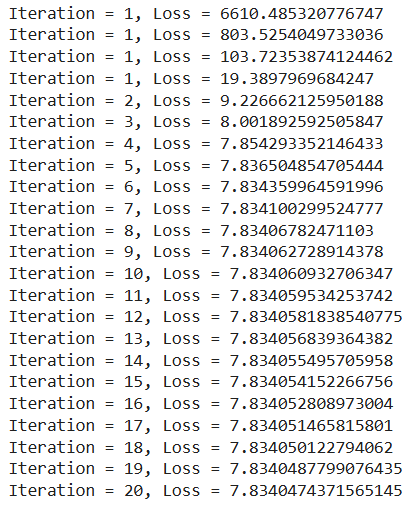
Model Training
Applications of Linear Regression
Linear regression is used in many different fields including finance, economics and psychology to understand and predict the behavior of a particular variable.
For example linear regression is widely used in finance to analyze relationships and make predictions. It can model how a company's earnings per share (EPS) influence its stock price. If the model shows that a 1increaseinEPSresultsina1 increase in EPS results in a 1increaseinEPSresultsina15 rise in stock price, investors gain insights into the company's valuation. Similarly, linear regression can forecast currency values by analyzing historical exchange rates and economic indicators, helping financial professionals make informed decisions and manage risks effectively.
Also read - Linear Regression - In Simple Words, with real-life Examples
Advantages and Disadvantages of Linear Regression
Advantages of Linear Regression
- Linear regression is a relatively simple algorithm, making it easy to understand and implement. The coefficients of the linear regression model can be interpreted as the change in the dependent variable for a one-unit change in the independent variable, providing insights into the relationships between variables.
- Linear regression is computationally efficient and can handle large datasets effectively. It can be trained quickly on large datasets, making it suitable for real-time applications.
- Linear regression is relatively robust to outliers compared to other machine learning algorithms. Outliers may have a smaller impact on the overall model performance.
- Linear regression often serves as a good baseline model for comparison with more complex machine learning algorithms.
- Linear regression is a well-established algorithm with a rich history and is widely available in various machine learning libraries and software packages.
Disadvantages of Linear Regression
- Linear regression assumes a linear relationship between the dependent and independent variables. If the relationship is not linear, the model may not perform well.
- Linear regression is sensitive to multicollinearity, which occurs when there is a high correlation between independent variables. Multicollinearity can inflate the variance of the coefficients and lead to unstable model predictions.
- Linear regression assumes that the features are already in a suitable form for the model. Feature engineering may be required to transform features into a format that can be effectively used by the model.
- Linear regression is susceptible to both overfitting and underfitting. Overfitting occurs when the model learns the training data too well and fails to generalize to unseen data. Underfitting occurs when the model is too simple to capture the underlying relationships in the data.
- Linear regression provides limited explanatory power for complex relationships between variables. More advanced machine learning techniques may be necessary for deeper insights.