Latent Text Analysis (lsa Package) Using Whole Documents in R (original) (raw)

Last Updated : 23 Jul, 2025

Latent Text Analysis (LTA) is a technique used to discover the hidden (latent) structures within a set of documents. This approach is instrumental in natural language processing (NLP) for identifying patterns, topics, and relationships in large text corpora. This article will explore using whole documents using the Isa Package in R programming language for Latent Text Analysis.

Understanding Latent Text Analysis

When performing Latent Text Analysis (LTA), treating the text as a whole document means that the analysis is done on the full text without breaking it down into smaller sub-components like paragraphs or sentences like research papers, customer feedback, Emails, News Articles, etc. This technique reduces the dimension of finding the underlying themes that are not usually visible.

Mathematical Significance of LSA

LSA uses Singular Value Decomposition (SVD) for analysis of the term-document matrix. The document term is divided into three components or matrices:

**A=UΣV T

where,

**U: An orthogonal matrix representing the term vectors.
**Σ: A diagonal matrix with singular values, representing the importance of each dimension.
**V: An orthogonal matrix representing the document vectors.
**T: This identifies the transpose of the orthogonal matrix.

Need for Latent Text Analysis?

LTA can be used for many purposes, some of which are:

**Uncover Hidden Patterns: Patterns and themes that are not visible can be identified by this method.
**Enhancing Data Insights: It helps in getting meaningful insights from the text document.
**Summarizing Large Text Corpora: For large collections of documents, summarizing the content into main topics or themes makes it easier to comprehend the overall structure and trends within the data.

lsa Package in R

The lsa package in R provides tools for performing Latent Semantic Analysis. It allows users to create a latent semantic space and perform various analyses such as term associations, document similarities, and topic modeling. The package integrates seamlessly with the "tm" package in R.

In this article, we will be using a fictional dataset and perform LTA on it. This article will contain news article information on different topics.

Step 1. Extract Data, Load, and Understand

In this step, we will create a fictional dataset and understand it before performing analysis on it.

R `

Fictional dataset of news articles

news_articles <- c( "The stock market is experiencing a significant downturn as inflation rates rise.", "Advances in artificial intelligence are revolutionizing various industries.", "Healthcare reform is a hot topic in the upcoming election.", "New developments in renewable energy technologies are promising for sustainability.", "The economy is showing signs of recovery with increased job growth.", "Artificial intelligence applications in healthcare are improving patient outcomes.", "The latest research in quantum computing has opened new possibilities in technology.", "Education reform is necessary to address the challenges faced by modern schools.", "Economic policies are being debated to tackle the effects of global trade imbalances.", "Advancements in biotechnology are leading to new treatments for chronic diseases." )

Categories for the articles

categories <- c("economy", "technology", "politics", "environment", "economy", "healthcare", "technology", "education", "politics", "healthcare")

Combine into a data frame

news_df <- data.frame(text = news_articles, category = categories, stringsAsFactors = FALSE)

Step 2. Preprocess the Text Data

Creating and Preprocessing the Corpus(a collection of words). The next step is to preprocess the text data by converting it to lowercase, removing punctuation, numbers, and stopwords, and stripping whitespace.

R `

Load required libraries

library(tm) library(SnowballC)

Create a text corpus

corpus <- Corpus(VectorSource(news_articles))

Preprocess the text data

corpus <- tm_map(corpus, content_transformer(tolower)) corpus <- tm_map(corpus, removePunctuation) corpus <- tm_map(corpus, removeNumbers) corpus <- tm_map(corpus, removeWords, stopwords("english")) corpus <- tm_map(corpus, stripWhitespace)

The corpus now consists of clean, preprocessed text data ready for analysis.

Step 3. Exploratory Data Analysis (EDA)

Now we will perform Exploratory Data Analysis (EDA) on our dataset.

**3.1: Creating a Term-Document Matrix

We create a Term-Document Matrix (TDM) which represents the frequency of terms in each document.

R `

Create a term-document matrix

tdm <- TermDocumentMatrix(corpus) tdm_matrix <- as.matrix(tdm) print(tdm_matrix)

**Output:

Docs
Terms 1 2 3 4 5 6 7 8 9 10
downturn 1 0 0 0 0 0 0 0 0 0
experiencing 1 0 0 0 0 0 0 0 0 0
inflation 1 0 0 0 0 0 0 0 0 0
market 1 0 0 0 0 0 0 0 0 0
rates 1 0 0 0 0 0 0 0 0 0
rise 1 0 0 0 0 0 0 0 0 0
significant 1 0 0 0 0 0 0 0 0 0
stock 1 0 0 0 0 0 0 0 0 0
advances 0 1 0 0 0 0 0 0 0 0
artificial 0 1 0 0 0 1 0 0 0 0
industries 0 1 0 0 0 0 0 0 0 0
intelligence 0 1 0 0 0 1 0 0 0 0
revolutionizing 0 1 0 0 0 0 0 0 0 0
various 0 1 0 0 0 0 0 0 0 0
election 0 0 1 0 0 0 1 0 0 0
healthcare 0 0 1 0 0 0 0 0 0 0
hot 0 0 1 0 0 0 0 0 0 0
reform 0 0 1 0 0 0 0 0 0 0
topic 0 0 1 0 0 0 0 0 0 0
upcoming 0 0 1 0 0 0 0 0 0 0
developments 0 0 0 1 0 0 0 0 0 0
energy 0 0 0 1 0 0 0 0 0 1
new 0 0 0 1 0 0 0 0 0 0
promising 0 0 0 1 0 0 0 0 0 0
renewable 0 0 0 1 0 0 0 0 0 1
sustainability 0 0 0 1 0 0 0 0 0 0
technologies 0 0 0 1 0 0 0 0 0 0
economy 0 0 0 0 1 0 0 0 0 0
growth 0 0 0 0 1 0 0 0 0 0
increased 0 0 0 0 1 0 0 0 0 0
job 0 0 0 0 1 0 0 0 0 0
recovery 0 0 0 0 1 0 0 0 0 0
showing 0 0 0 0 1 0 0 0 0 0
signs 0 0 0 0 1 0 0 0 0 0
area 0 0 0 0 0 1 0 0 0 0
companies 0 0 0 0 0 1 0 0 0 0
continues 0 0 0 0 0 1 0 0 0 0
focus 0 0 0 0 0 1 0 0 0 0
key 0 0 0 0 0 1 0 0 0 0
tech 0 0 0 0 0 1 0 0 0 0
approaches 0 0 0 0 0 0 1 0 0 0
day 0 0 0 0 0 0 1 0 0 0
debates 0 0 0 0 0 0 1 0 0 0
heating 0 0 0 0 0 0 1 0 0 0
political 0 0 0 0 0 0 1 0 0 0
advancements 0 0 0 0 0 0 0 1 0 0
automotive 0 0 0 0 0 0 0 1 0 0
driving 0 0 0 0 0 0 0 1 0 0
forward 0 0 0 0 0 0 0 1 0 0
industry 0 0 0 0 0 0 0 1 0 0
technological 0 0 0 0 0 0 0 1 0 0
economic 0 0 0 0 0 0 0 0 1 0
horizon 0 0 0 0 0 0 0 0 1 0
indicators 0 0 0 0 0 0 0 0 1 0
may 0 0 0 0 0 0 0 0 1 0
recession 0 0 0 0 0 0 0 0 1 0
suggest 0 0 0 0 0 0 0 0 1 0
becoming 0 0 0 0 0 0 0 0 0 1
costeffective 0 0 0 0 0 0 0 0 0 1
sources 0 0 0 0 0 0 0 0 0 1

The TDM matrix shows the frequency of each term in each document.

**3.2: Plot the most frequent terms

Lets plot the most frequent terms of our whole document to understand it better.

R `

Plot the most frequent terms

library(ggplot2) term_freq <- sort(rowSums(tdm_matrix), decreasing = TRUE) term_freq_df <- data.frame(term = names(term_freq), freq = term_freq)

ggplot(term_freq_df[1:10,], aes(x = reorder(term, -freq), y = freq)) + geom_bar(stat = "identity") + labs(title = "Top 10 Most Frequent Terms", x = "Terms", y = "Frequency") + theme_minimal()

**Output:

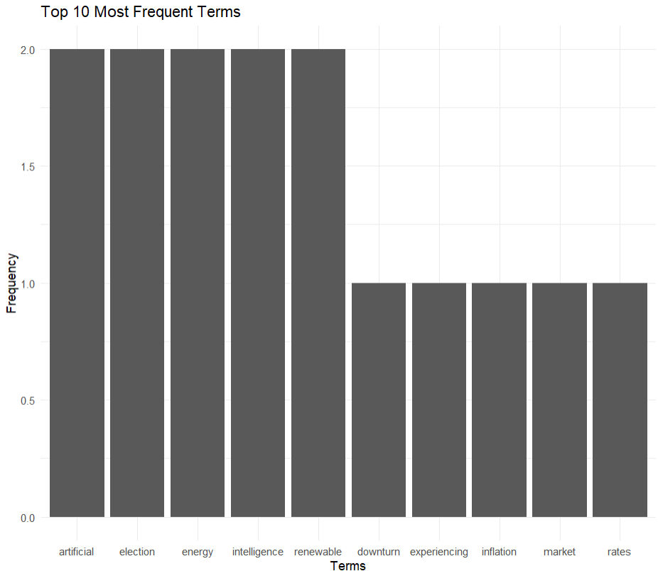
mostfrequentgfg

Most frequent words

**3.3: Visualizing Word Frequencies with a Word Cloud

We visualize word frequencies using a word cloud to identify the most frequent terms in the corpus.

R `

EDA: Create a word cloud

library(wordcloud) library(RColorBrewer)

word_freqs <- sort(rowSums(tdm_matrix), decreasing = TRUE) word_freqs_df <- data.frame(word = names(word_freqs), freq = word_freqs) wordcloud(words = word_freqs_df$word, freq = word_freqs_df$freq, min.freq = 1, colors = brewer.pal(8, "Dark2"), scale = c(3, 0.5))

**Output:

WORDCLOUDGFG

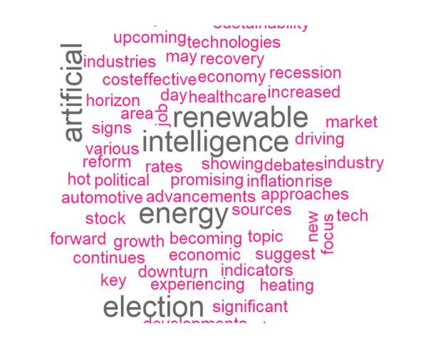
WORD CLOUD

The word cloud highlights the most frequent words in the dataset, providing a quick visual summary of the corpus content.

**3.4: Plotting a Heatmap of the Term-Document Matrix

We plot a heatmap to show the distribution of terms across documents.

R `

EDA: Plot a heatmap of the term-document matrix

library(pheatmap)

pheatmap(tdm_matrix, cluster_rows = TRUE, cluster_cols = TRUE, main = "Heatmap of Term-Document Matrix")

**Output:

heatmapgfg

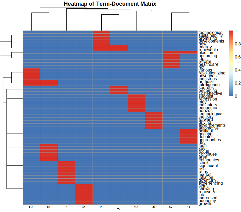
HEATMAP

The heatmap displays the term frequencies across documents, with clustering indicating groups of similar terms and documents.

**3.5: Plotting Singular Values to Show Relative Importance of Components

We perform Singular Value Decomposition (SVD) to identify the importance of each component.

R `

Perform Singular Value Decomposition (SVD)

svd_result <- svd(tdm_matrix) singular_values <- svd_result$d

Plot the singular values

plot(singular_values, type = "o", main = "Singular Values", xlab = "Component", ylab = "Singular Value")

**Output:

singlevaluegfg

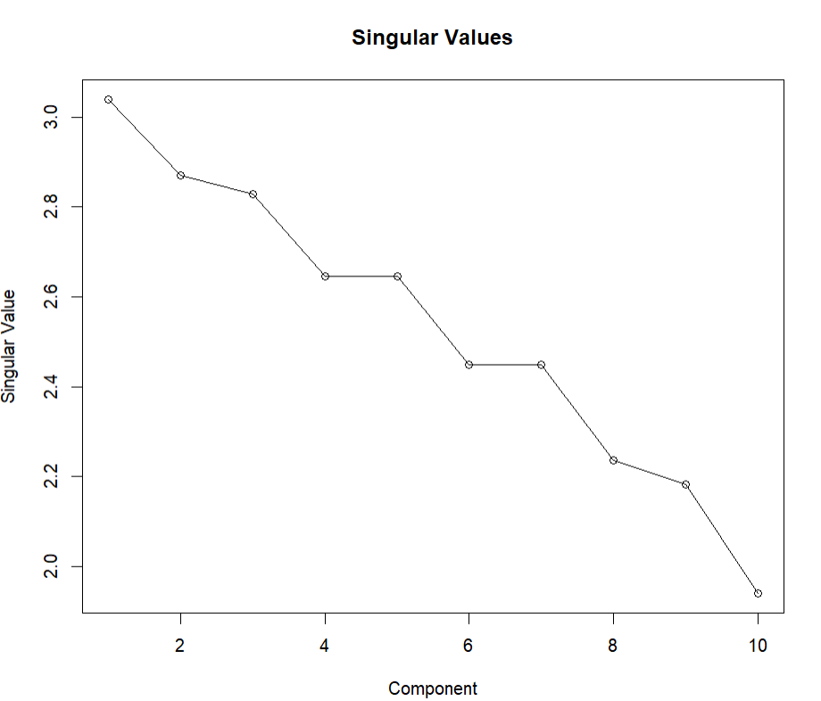
singular value

Step 4. Perform Latent Semantic Analysis (LSA)

We perform LSA on the TDM matrix to reduce its dimensionality and extract meaningful patterns. We extract the top and bottom terms for each LSA component to understand the main topics represented.

R `

Perform LSA

library(lsa)

lsa_space <- lsa(tdm_matrix)

Convert LSA space to matrix and extract the document coordinates

lsa_matrix <- as.textmatrix(lsa_space) doc_coords <- as.data.frame(lsa_matrix[, 1:2]) # Reduce to 2 dimensions for visualization

Add column names for LSA dimensions

colnames(doc_coords) <- c("Dim1", "Dim2")

Extract top and bottom terms for each component

terms <- rownames(lsa_matrix) components <- lsa_space$tk

top_terms <- function(component, terms, num = 5) { sorted <- sort(component, decreasing = TRUE) top <- terms[order(component, decreasing = TRUE)[1:num]] bottom <- terms[order(component, decreasing = FALSE)[1:num]] list(top = top, bottom = bottom) }

for (i in 1:2) { cat("Component", i, "\n") terms_i <- top_terms(components[, i], terms) cat("Top terms: ", terms_i$top, "\n") cat("Bottom terms: ", terms_i$bottom, "\n\n") }

**Output:

Component 1
Top terms: election hot topic upcoming healthcare
Bottom terms: new computing latest opened possibilities

Component 2
Top terms: artificial intelligence healthcare reform applications
Bottom terms: developments energy new promising renewable

This reveals the key terms for each topic.

Conclusion

In this article, we discussed how to use Isa package in R for Latent Text Analysis for a whole document. We used multiple graphs to visualize our data and processing. We also learnt how to use other packages to perform analysis over a news article to find sub topics and frequent words.