NumPy Array Broadcasting (original) (raw)

Last Updated : 17 Jan, 2025

Broadcasting simplifies **mathematical operations on arrays with different shapes. It enables NumPy to efficiently apply operations element-wise without explicitly copying or reshaping data.

It automatically **adjusts the smaller array to match the shape of the larger array by replicating its values along the necessary dimensions. This feature reduces memory usage and eliminates the need for manual loops making code concise and computationally faster making it essential for handling large datasets and performing complex calculations in python. Let’s understand the concept with quick example: **Suppose we want to add scalar to a 2D Array.

Python `

import numpy as np

array_2d = np.array([[1, 2, 3], [4, 5, 6]]) # 2D array scalar = 10 # Scalar value

result = array_2d + scalar print(result)

`

Output

[[11 12 13] [14 15 16]]

Here, scalar 10 is “broadcast” to match the shape of the 2D array and each element of array_2d has 10 added to it.

How Broadcasting Works in NumPy?

Broadcasting applies specific rules to determine whether two arrays can be aligned for operations:

1. **Check Dimensions: Ensure the arrays have the same number of dimensions or expandable dimensions.
2. **Dimension Padding: If arrays have different numbers of dimensions, the smaller array is left-padded with ones.
3. **Shape Compatibility: Two dimensions are compatible if:
   • They are equal, or
   • One of them is 1.

If these conditions are not met, a ValueError is raised.

**Practical Examples of Broadcasting

**Example 1 : Broadcasting Array in Single Value and 1D Addition

The code creates a NumPy array arr with values [1, 2, 3]. It adds 1 to each element using broadcasting, resulting in [2, 3, 4], and prints the updated array.

Python `

import numpy as np arr = np.array([1, 2, 3])

res = arr + 1 # Adds 1 to each element print(res)

`

Example 2 : Broadcasting Array in 1D and 2D Addition

This code demonstrates **broadcasting in NumPy, where a 1D array (a1) is added to a 2D array (a2). Here’s a brief explanation: NumPy automatically expands a1 along the rows to match the shape of a2. This shows how NumPy simplifies operations between arrays of different shapes by stretching smaller arrays

Python `

import numpy as np

Broadcasting a 1D array with a 2D array

a1 = np.array([2, 4, 6]) a2 = np.array([[1, 3, 5], [7, 9, 11]]) res = a1 + a2 print(res)

`

Output

[[ 3 7 11] [ 9 13 17]]

Example 3: **Using Broadcasting for Matrix Multiplication

The example demonstrates how each element of the matrix is multiplied by the corresponding element in the broadcasted vector:

Python `

import numpy as np matrix = np.array([[1, 2], [3, 4]]) vector = np.array([10, 20]) result = matrix * vector print(result)

`

**Example 4: Scaling Data with Broadcasting

To better understand broadcasting, let’s consider a real-world example: **counting calories in foods based on their macro-nutrient breakdown. Foods contain fats, proteins, and carbohydrates, each contributing a specific caloric value per gram:

• **Fats: 9 calories per gram (CPG)
• **Proteins: 4 CPG
• **Carbohydrates: 4 CPG

Suppose we have a dataset where each row represents a food item, and the columns represent the grams of fats, proteins, and carbs. To compute the caloric breakdown for each food, we multiply each nutrient by its respective caloric value. This is where NumPy broadcasting simplifies the process.

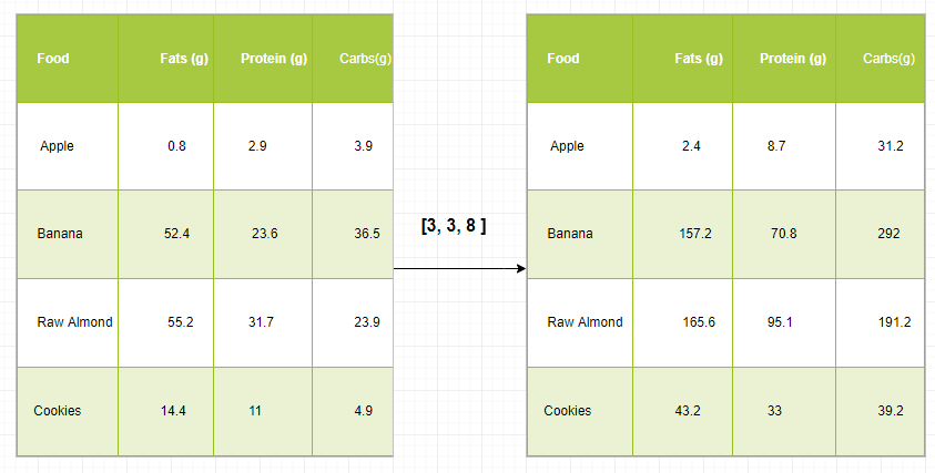
Left table shows the original data with food items and their respective grams of fats, proteins, and carbs. The array “[3, 3, 8]” represents the caloric values per gram for fats, proteins, and carbs respectively. This array is being broadcast to match the dimensions of the original data and arrow indicates the broadcasting operation.

• The broadcasting array is multiplied element-wise with each row of the original data.
• As a result, right table shows the result of the multiplication, where each cell represents the caloric contribution of that specific nutrient in the food item. Python `

import numpy as np food_data = np.array([[0.8, 2.9, 3.9], [52.4, 23.6, 36.5], [55.2, 31.7, 23.9], [14.4, 11, 4.9]])

Caloric values per gram

caloric_values = np.array([3, 3, 8])

Broadcast caloric values to match food data

caloric_matrix = caloric_values

Calculate calorie breakdown for each food

calorie_breakdown = food_data * caloric_matrix print(calorie_breakdown)

`

Output

[[ 2.4 8.7 31.2] [157.2 70.8 292. ] [165.6 95.1 191.2] [ 43.2 33. 39.2]]

The example demonstrates how broadcasting eliminates the need for explicit loops to scale data. It’s efficient and concise—a critical feature when working with large datasets.

Below are some more practical examples and use cases showcasing its versatility.

**Example 5: Adjusting Temperature Data Across Multiple Locations

Suppose you have a 2D array (temperatures) representing daily temperature readings across multiple cities (rows: cities, columns: days). You want to adjust these temperatures by adding a specific correction factor for each city.

Python `

import numpy as np

temperatures = np.array([ [30, 32, 34, 33, 31],
[25, 27, 29, 28, 26], [20, 22, 24, 23, 21]
])

Correction factors for each city

corrections = np.array([1.5, -0.5, 2.0])

adjusted_temperatures = temperatures + corrections[:, np.newaxis] print(adjusted_temperatures)

`

Broadcasting eliminates the need for manual loops to adjust data for each city individually.

**Example 6: Normalizing Image Data

Normalization is crucial in many real-world scenarios like image processing and machine learning because it:

1. Centers data by subtracting the mean, ensuring features have zero mean.
2. Scales data by dividing by the standard deviation, ensuring features have unit variance.
3. Improves numerical stability and performance of algorithms like gradient descent.

Let’s demonstrate how broadcasting simplifies normalization without requiring explicit loops.

Python `

import numpy as np

Example image data (3x3 grayscale image)

image = np.array([ [100, 120, 130], [90, 110, 140], [80, 100, 120] ])

mean = image.mean(axis=0) # Mean per column (feature-wise) std = image.std(axis=0) # Standard deviation per column

Normalize using broadcasting

normalized_image = (image - mean) / std print(normalized_image)

`

Output

[[ 1.22474487 1.22474487 0. ] [ 0. 0. 1.22474487] [-1.22474487 -1.22474487 -1.22474487]]

Example 7: **Centering Data in Machine Learning

Broadcasting simplifies feature-wise operations crucial in machine learning workflows.

Python `

import numpy as np

data = np.array([ [10, 20], [15, 25], [20, 30] ])

feature_mean = data.mean(axis=0)

Center data using broadcasting

centered_data = data - feature_mean print(centered_data)

`

Output

[[-5. -5.] [ 0. 0.] [ 5. 5.]]