Python | Visualizing image in different color spaces (original) (raw)

Last Updated : 04 Jan, 2023

OpenCV (Open Source Computer Vision) is a computer vision library that contains various functions to perform operations on pictures or videos. It was originally developed by Intel but was later maintained by Willow Garage and is now maintained by Itseez. This library is cross-platform that is it is available on multiple programming languages such as Python, C++ etc.

Let’s discuss different ways to visualize images where we will represent images in different formats like grayscale, RGB scale, Hot_map, edge map, Spectral map, etc.

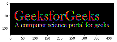
RGB Image :

RGB image is represented by linear combination of 3 different channels which are R(Red), G(Green) and B(Blue). Pixel intensities in this color space are represented by values ranging from 0 to 255 for single channel. Thus, number of possibilities for one color represented by a pixel is 16 million approximately [255 x 255 x 255 ].

import cv2

import matplotlib.pyplot as plt

img = cv2.imread( 'g4g.png' )

plt.imshow(img)

Output :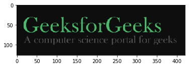

Gray Scale Image :

Grayscale image contains only single channel. Pixel intensities in this color space is represented by values ranging from 0 to 255. Thus, number of possibilities for one color represented by a pixel is 256.

import cv2

img = cv2.imread( 'g4g.png' , 0 )

img = cv2.cvtColor(img, cv2.COLOR_BGR2GRAY)

cv2.imshow( 'image' , img)

cv2.waitKey( 0 )

cv2.destroyAllWindows()

Output :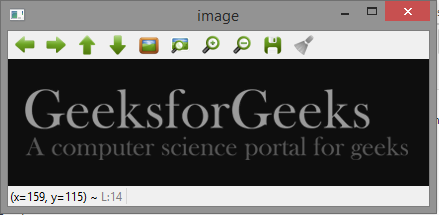

YCrCb Color Space :

Y represents Luminance or Luma component, Cb and Cr are Chroma components. Cb represents the blue-difference (difference of blue component and Luma Component). Cr represents the red-difference (difference of red component and Luma Component).

import cv2

img = cv2.imread( 'g4g.png' )

img = cv2.cvtColor(img, cv2.COLOR_BGR2YCrCb)

cv2.imshow( 'image' , img)

cv2.waitKey( 0 )

cv2.destroyAllWindows()

Output :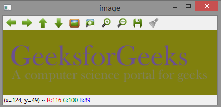

HSV color space :

H : Hue represents dominant wavelength.
S : Saturation represents shades of color.
V : Value represents Intensity.

import cv2

img = cv2.imread( 'g4g.png' )

img = cv2.cvtColor(img, cv2.COLOR_BGR2HSV)

cv2.imshow( 'image' , img)

cv2.waitKey( 0 )

cv2.destroyAllWindows()

Output :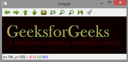

LAB color space :

L – Represents Lightness.
A – Color component ranging from Green to Magenta.
B – Color component ranging from Blue to Yellow.

import cv2

img = cv2.imread( 'g4g.png' )

img = cv2.cvtColor(img, cv2.COLOR_BGR2LAB)

cv2.imshow( 'image' , img)

cv2.waitKey( 0 )

cv2.destroyAllWindows()

Output :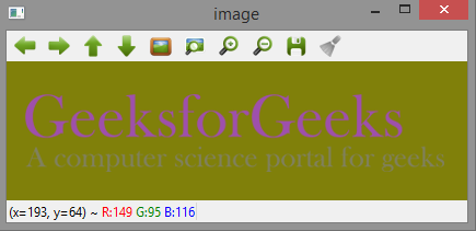

Edge map of image :

Edge map can be obtained by various filters like laplacian, sobel, etc. Here, we use Laplacian to generate edge map.

import cv2

img = cv2.imread( 'g4g.png' )

laplacian = cv2.Laplacian(img, cv2.CV_64F)

cv2.imshow( 'EdgeMap' , laplacian)

cv2.waitKey( 0 )

cv2.destroyAllWindows()

Output :

Heat map of image :

In Heat map representation, individual values contained in a matrix are represented as colors.

import matplotlib.pyplot as plt

import cv2

img = cv2.imread( 'g4g.png' )

plt.imshow(img, cmap = 'hot' )

Output :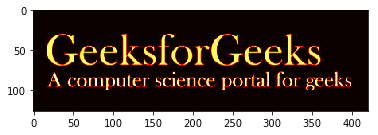

Spectral Image map :

Spectral Image map obtains the spectrum for each pixel in the image of a scene.

import matplotlib.pyplot as plt

import cv2

img = cv2.imread( 'g4g.png' )

plt.imshow(img, cmap = 'nipy_spectral' )

Output :