Complete Guide To SARIMAX in Python (original) (raw)
Time series data consists of observations collected over time at equally spaced intervals. SARIMAX is a statistical model designed to capture and forecast the underlying patterns, trends, and seasonality in such data. In this article, we'll explore the SARIMAX model, understand its mathematical underpinnings, and explore its practical applications.
What is Sarimax?
The Seasonal Autoregressive Integrated Moving Average with Exogenous Regressors (SARIMAX) model is a powerful time series forecasting technique that extends the traditional ARIMA model to account for **seasonality and external factors. It's a versatile model that can accommodate both autoregressive (AR) and moving average (MA) components, integrate differencing to make the data stationary, and incorporate external variables or regressors. SARIMAX is particularly valuable when dealing with time-dependent data that exhibits recurring patterns over specific time intervals.
Components of SARIMAX
- **Seasonal Component (S): Captures the periodic patterns in the data, such as weekly, monthly, or yearly cycles.
- **Autoregressive Component (AR): Represents the relationship between the current value and previous values in the time series.
- **Integrated Component (I): Involves differencing to make the time series stationary by removing trends and seasonality.
- **Moving Average Component (MA): Accounts for the dependency of the current value on past error terms, used to calculate trend.
- **Exogenous Regressors (X): Allows the inclusion of external variables that may affect the time series.
What is seasonality?
Seasonality in time series data refers to recurring and predictable patterns that occur at regular intervals over time. These patterns can manifest in various forms, such as daily, weekly, monthly, or yearly cycles, and are often influenced by external factors like weather, holidays, or economic seasons. The presence of seasonality implies that there are systematic variations in the data that repeat within specific time frames.
For example, retail sales may exhibit seasonality with higher activity during holiday seasons, or energy consumption might show seasonality with increased demand during winter or summer months. Seasonal patterns can significantly impact the overall trend of a time series and need to be identified and accounted for in forecasting models.
Understanding seasonality is crucial for accurate predictions because it helps capture the cyclic nature of the data. Analysts use various statistical techniques to detect and model seasonality, allowing them to make more informed decisions and forecasts. Seasonal decomposition, Fourier analysis, and autocorrelation functions are common tools employed to analyze and address seasonality in time series data. By acknowledging and incorporating these repetitive patterns, forecasting models like SARIMAX can better capture the inherent structure of the data and provide more reliable predictions.
Why is it important to handle seasonality?
Handling seasonality in time series data is crucial for accurate forecasting and decision-making. Seasonal patterns introduce regular fluctuations in the data, and failing to account for them can lead to inaccurate predictions and suboptimal business decisions. Moreover, It impacts consumer behavior, and businesses need to align their strategies accordingly. Handling seasonality provides insights into when to launch promotions, adjust pricing, or introduce new products, enabling more informed decision-making. Seasonal fluctuations can affect cash flow, revenue, and profitability. Effective handling of seasonality supports better financial planning, helping businesses manage budgets, cash reserves, and investment decisions throughout the year.
How to handle Seasonality?
Handling seasonality in time series data involves modeling and incorporating the recurring patterns observed at regular intervals. Imagine you have daily data on ice cream sales, and you notice a seasonal pattern where sales tend to increase during the summer months and decrease during the winter months. To handle this seasonality, you can use a SARIMAX model in following steps:
Step 1: **Differencing (Integration):
Seasonal patterns can make the data non-stationary. Apply differencing if needed to make the series stationary. This might involve taking the first difference or applying a seasonal difference, depending on the characteristics of your data.
Seasonal differencing is often applied to make the time series stationary. The differencing parameter is denoted as d for seasonal differencing.
Differencing involves subtracting the time series from a lagged version of itself. The d-th differencing can be represented as:
Y_t' = Y_t - Y_t-d
Here,Y_t' is the differenced series, and is the seasonal period.
**Step 2: Identify Seasonal Component
SARIMAX accounts for seasonality in the time series. Seasonal differences are modeled through the inclusion of seasonal autoregressive (SAR) and seasonal moving average (SMA) terms. These terms capture the repeating patterns in the data over specific time intervals (seasons).
To identify the seasonal component of a time series, we can use various decomposition techniques. One common approach is to use the Seasonal-Trend decomposition using LOESS (STL)****.**This helps in identifying the trend, seasonal, and residual components. These components, can help identify recurring patterns at regular intervals, to understand the model better.
**Trend
Compute the moving average to capture the trend. We can use a simple moving average or other techniques like exponential smoothing. Here, we're using moving average.
The moving average is computed by taking the average of the values over a specified number of periods, which is m in this case.
SMA(t) = (Y_{t-k+1} + ... + Y_t) / k
- Where, Y_t the value at time t****.**
- **k is the number of periods in the moving average.
It is particularly useful for removing short-term fluctuations and highlighting the overall direction of the data.
**Compute Detrended Series
Subtract the moving average from the original time series to obtain a detrended series.
Detrended Series= y_t - Moving Average
**Calculate the Seasonal Component
The seasonal component represents the average pattern or deviation from the overall trend that occurs in each season across multiple years. It helps identify recurring patterns or cycles that are not part of the long-term trend.
\text{Seasonal Component} = \frac{1}{n} \sum_{j=1}^{n} \text{Detrended Series}_{j}
Where, n be the number of seasons.
The choice of n depends on the periodicity of the seasonality in the data. For example, if you observe a yearly seasonality, n would be set to 12 for monthly data.
**Calculate Residuals
Residuals represent the remaining variation in the time series after accounting for both the trend and the seasonal component.
Residuals=Detrended Series−Seasonal Component
It helps defining the unexplained variation or noise in the time series data Residuals are important for model diagnostics and validation. A good forecasting model should have residuals that are random and show no discernible pattern. If patterns are present in the residuals, it suggests that the model may need further refinement.
The SARIMAX Model
Putting it all together, the SARIMAX (p,d,q)(P,Q,Ds,) model can be expressed as:
\Theta(L)^{p} \theta(L^{s})^{P} \Delta^{d} \Delta_{s}^{D} y_{t} = \Phi(L)^{q} \phi(L^{s})^{Q} \Delta^{d} \Delta_{s}^{D} \epsilon_{t} + \sum_{i=1}^{n} \beta_{i} x^{i}_{t}
-\Theta(L)^{p} \theta(L^{s})^{P} \Delta^{d} \Delta_{s}^{D} y_{t} : represents the dependent variable, denoted as \(y_{t}\), which is likely a time series variable.
where,
- The terms \Theta(L)^{p} \theta(L^{s})^{P} involves autoregressive (AR) and seasonal autoregressive components, respectively. \\Delta^{d} \Delta_{s}^{D} denote differencing, commonly used to achieve stationarity in time series data.
- \epsilon_{t} represents the error term of the model.
- \sum_{i=1}^{n} \beta_{i} x^{i}_{t} includes (n) exogenous variables x^{i}_{t} with corresponding coefficients \beta_{i}
In summary, this SARIMAX model combines autoregressive and seasonal autoregressive components, differencing for stationarity, and includes exogenous variables to capture additional factors influencing the dependent variable over time.
Effect of choice of parameters on the SARIMAX model
Order of Differencing (d and D)
- **Over-Differencing: Too much differencing can lead to a series that is overly stationary, potentially losing valuable information. If the original time series already exhibits a stable trend, applying too much differencing (d or D values that are too high) may remove the trend and make the data less interpretable.
- **Under-Differencing: Insufficient differencing may result in a non-stationary series, leading to inaccuracies in model estimation. If the time series has a clear trend or seasonality, not differencing the data appropriately (d or D values too low) can result in a model that fails to capture these patterns.
Seasonal and Non-Seasonal AR Terms (p and P)
- **Too Many AR Terms (p or P: Including too many autoregressive terms may lead to overfitting, capturing noise as if it were a real pattern. If a monthly time series is modeled with a high number of autoregressive terms, the model may pick up on short-term fluctuations that do not represent the underlying structure.
- **Too Few AR Terms (p or P: Insufficient autoregressive terms may result in the model failing to capture important dependencies between past and present observations. If a time series has strong autocorrelation in the past, not including enough autoregressive terms can lead to poor predictive performance.
**Seasonal and Non-Seasonal MA Terms (q and Q)
- **Too Many MA Terms (q or Q): Including too many moving average terms can result in a model that is too responsive to short-term fluctuations, leading to overfitting. In a highly seasonal dataset, too many moving average terms may try to fit noise as if it were a real pattern, leading to less reliable forecasts.
- **Too Few MA Terms (q or Q: Insufficient moving average terms may result in a failure to capture short-term fluctuations, especially in the presence of noise. If the time series has short-term variations that are not accounted for, the model may struggle to adapt to sudden changes in the data.
**Seasonal Period (m)
- **Incorrect Seasonal Period: Choosing an incorrect seasonal period can lead to the model trying to capture patterns that do not exist in the data. If the seasonal period is mistakenly set to 6 months when the actual pattern repeats every 12 months, the model may misinterpret the seasonality.
- **Omitting Seasonal Component If the time series exhibits clear seasonality, neglecting to include a seasonal component can result in a model that fails to capture important patterns. Monthly sales data often exhibits seasonality, and omitting a seasonal component may lead to suboptimal forecasts.
Python Implementation of Sarimax Model
Let's delve more into the topic with python implementation using dataset: Air Passenger dataset.
**Step 1: Importing Libraries
Import necessary libraries for working with time series data, plotting, and statistical models. 'pmdarima' is used for automated ARIMA modeling.
Python3 `
from datetime import datetime import numpy as np import pandas as pd import matplotlib.pylab as plt %matplotlib inline from matplotlib.pylab import rcParams
from statsmodels.tsa.stattools import adfuller !pip install pmdarima -q import pmdarima as pm from statsmodels.tsa.seasonal import seasonal_decompose
`
**Step 2: Data Loading and Data formatting
Read the AirPassengers dataset from the provided URL into a Pandas DataFrame.
Python3 `
df = pd.read_csv("https://raw.githubusercontent.com/AileenNielsen/TimeSeriesAnalysisWithPython/master/data/AirPassengers.csv")
`
Convert the 'Month' column to datetime format and set it as the index of the DataFrame.
Python3 `
df['Month'] = pd.to_datetime(df['Month'], infer_datetime_format=True) df = df.set_index(['Month'])
`
**Step 3: Differencing
Python3 `
df['#Passengers_diff'] = df['#Passengers'].diff(periods=12) df.info()
`
**Output:
<class 'pandas.core.frame.DataFrame'>
DatetimeIndex: 144 entries, 1949-01-01 to 1960-12-01
Data columns (total 2 columns):
Column Non-Null Count Dtype
0 #Passengers 144 non-null int64
1 #Passengers_diff 132 non-null float64
dtypes: float64(1), int64(1)
memory usage: 3.4 KB
Differencing involves subtracting a lagged version of the time series from itself. In the case of seasonal differencing, you subtract the value from the same season in the previous year.
When you take the first seasonal difference, you lose the first 12 data points (since there is no previous year's data for the first 12 months). This leads to missing values in the resulting differenced series.
Python3 `
df['#Passengers_diff'].fillna(method='backfill', inplace=True)
`
**Output:
<class 'pandas.core.frame.DataFrame'>
DatetimeIndex: 144 entries, 1949-01-01 to 1960-12-01
Data columns (total 2 columns):
Column Non-Null Count Dtype
0 #Passengers 144 non-null int64
1 #Passengers_diff 144 non-null float64
dtypes: float64(1), int64(1)
memory usage: 3.4 KB
**Step 4: Identify Seasonal Component
Python3 `
result = seasonal_decompose(df['#Passengers'], model='multiplicative', period=12) trend = result.trend.dropna() seasonal = result.seasonal.dropna() residual = result.resid.dropna()
Plot the decomposed components
plt.figure(figsize=(6,6))
plt.subplot(4, 1, 1) plt.plot(df['#Passengers'], label='Original Series') plt.legend()
plt.subplot(4, 1, 2) plt.plot(trend, label='Trend') plt.legend()
plt.subplot(4, 1, 3) plt.plot(seasonal, label='Seasonal') plt.legend()
plt.subplot(4, 1, 4) plt.plot(residual, label='Residuals') plt.legend()
plt.tight_layout() plt.show()
`
**Output:
.png)
Decomposition
- The top subplot shows the original time series, which represents the monthly passenger counts over time.
- The second subplot displays the trend component extracted from the original series. The trend represents the long-term movement or pattern in the data, smoothing out short-term fluctuations helping to identify the overall direction of the time series.
- The third subplot represents the seasonal component, capturing the repeating patterns or cycles in the data that occur at regular intervals indicating monthly seasonality helping to understand the regular fluctuations that happen at specific times each year.
- The bottom subplot shows the residuals or the remainder after removing the trend and seasonal components.
**Step 5: Exogenous variable
Create an exogenous variable 'month_index' representing the month from the datetime index. This will be used as an exogenous variable in the SARIMAX model.
Python3 `
df['month_index'] = df.index.month
`
**Step 6: SARIMAX Model Fitting
Use pmdarima to automatically fit a Seasonal AutoRegressive Integrated Moving Average with eXogenous variables (SARIMAX) model to the 'AirPassengers' data. The parameters are set for automatic selection based on the Akaike Information Criterion (AIC) through the 'auto_arima' function.
Python3 `
SARIMAX_model = pm.auto_arima(df[['#Passengers']], exogenous=df[['month_index']], start_p=1, start_q=1, test='adf', max_p=3, max_q=3, m=12, start_P=0, seasonal=True, d=None, D=1, trace=False, error_action='ignore', suppress_warnings=True, stepwise=True)
`
**Step 7: SARIMAX forecasting function
Define a function sarimax_forecast that takes a trained SARIMAX model and generates forecasts for a specified number of periods (24 months in this case). It also plots the original time series, the forecast, and the confidence intervals.
Python3 `
def sarimax_forecast(SARIMAX_model, periods=24): # Forecast n_periods = periods
forecast_df = pd.DataFrame({"month_index": pd.date_range(df.index[-1], periods=n_periods, freq='MS').month},
                           index=pd.date_range(df.index[-1] + pd.DateOffset(months=1), periods=n_periods, freq='MS'))

fitted, confint = SARIMAX_model.predict(n_periods=n_periods,
                                        return_conf_int=True,
                                        exogenous=forecast_df[['month_index']])
index_of_fc = pd.date_range(df.index[-1] + pd.DateOffset(months=1), periods=n_periods, freq='MS')

# make series for plotting purpose
fitted_series = pd.Series(fitted, index=index_of_fc)
lower_series = pd.Series(confint[:, 0], index=index_of_fc)
upper_series = pd.Series(confint[:, 1], index=index_of_fc)

# Plot
plt.figure(figsize=(15, 7))
plt.plot(df["#Passengers"], color='#1f76b4')
plt.plot(fitted_series, color='darkgreen')
plt.fill_between(lower_series.index,
                 lower_series,
                 upper_series,
                 color='k', alpha=.15)

plt.title("SARIMAX - Forecast of Airline Passengers")
plt.show()
`
**Step 6: Forecasting
Call the 'sarimax_forecast' function with the trained SARIMAX model and specify the number of periods (here, 24 months) for forecasting. The function will generate the forecast plot based on the SARIMAX model.
Python3 `
sarimax_forecast(SARIMAX_model, periods=24)
`
Output:
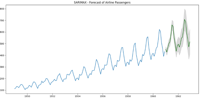
In, the plot shaded region is indicating the confidence interval around the predicted values.
Conclusion
In this example, we've introduced an exogenous variable by adding the month number, even though seasonality already captures monthly patterns.
Despite this seemingly redundant addition, the model demonstrates impressive predictive performance. The narrow width of the forecasted confidence interval indicates a high level of confidence in the model's predictions. In simpler terms, the model seems to be quite certain about its forecasts, and the predictions align well with the observed data.