Dynamic Programming in Python (original) (raw)
Dynamic Programming (DP) is a technique used to solve problems by breaking them into smaller subproblems and storing their results for later use.
- It avoids solving the same subproblem multiple times.
- It is commonly used in optimization and counting problems.
- DP can be implemented using Memoization (Top-Down) or Tabulation (Bottom-Up).
Use of Dynamic Programming
In the recursion tree for the Fibonacci example, the same subproblems appear repeatedly. For instance, values such as F(2), F(3) and F(4) are recomputed multiple times. This repeated work causes the naive recursive solution to grow exponentially in time as n becomes larger.
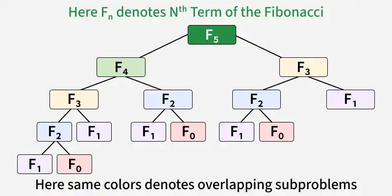
Recursion Tree for F5 with Overlapping Subproblems
Dynamic Programming improves this by solving each subproblem once and reusing the stored result.
- **Identify Subproblems: Break the main problem into smaller subproblems such as F(n-1) and F(n-2).
- **Store Solutions: Save the result of each solved subproblem in a table, array or cache.
- **Build the final answer: Compute larger values using the stored results of smaller subproblems.
- **Avoid Recomputation: Once a subproblem (for example F(2)) has been solved, its stored value is reused instead of being calculated again.
Approaches of Dynamic Programming (DP)
Dynamic Programming can be implemented using two main approaches:
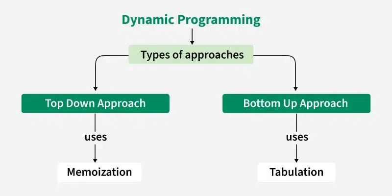
Approaches of Dynamic Programming (DP)
1. Top-Down Approach (Memoization)
In the top-down approach, we start with the original problem and solve smaller subproblems recursively. The results of solved subproblems are stored so they can be reused when needed again.
- Uses recursion to break the problem into smaller subproblems.
- Stores previously computed results in a memoization table.
- Avoids repeated calculations by reusing stored values.
2. Bottom-Up Approach (Tabulation)
In the bottom-up approach, we solve the smallest subproblems first and use their results to build the solution for larger subproblems.
- Uses iteration instead of recursion.
- Stores results in a DP table starting from the base cases.
- Builds the final solution step by step using previously computed values.
To know more about DP, refer to this article When to Use Dynamic Programming (DP)
Example of Dynamic Programming (DP)
Let's understand Dynamic Programming using the Fibonacci Sequence, where each number is the sum of the previous two numbers. Fibonacci Sequence:
0, 1, 1, 2, 3, 5, 8, 13, 21, 34, ...
The Fibonacci formula is:
F(n) = F(n - 1) + F(n - 2)
Where:
- F(0) = 0
- F(1) = 1
Brute Force Approach
A simple recursive solution calculates each Fibonacci number by repeatedly computing the previous two Fibonacci numbers.
Python `
def fib(n): if n <= 1: return n return fib(n - 1) + fib(n - 2)
print(fib(5))
`
Below is the recursion tree of the above recursive solution:
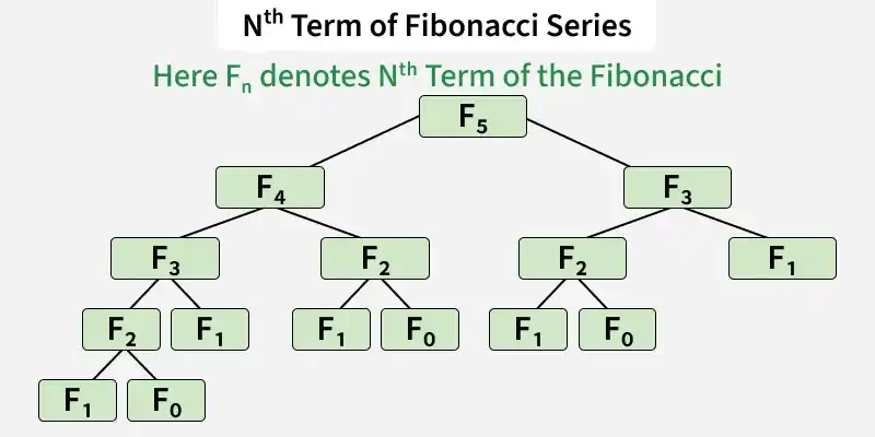
nth term of fibonacci series
Using Memoization Approach – O(n) Time and O(n) Space
In the memoization approach, we use recursion along with a memoization array (memo) to store already calculated Fibonacci values. Before solving a subproblem, we first check whether its result is already available in the array. If it is available, we reuse it directly; otherwise, we calculate it and store the result for future use.
Python `
def fib_rec(n, memo): if n <= 1: return n
if memo[n] != -1:
    return memo[n]

memo[n] = fib_rec(n - 1, memo) + fib_rec(n - 2, memo)
return memo[n]
def fib(n): memo = [-1] * (n + 1) return fib_rec(n, memo)
n = 5 print(fib(n))
`
**Explanation:
- memo = [-1] * (n + 1) creates a memoization array initialized with -1.
- if memo[n] != -1 checks whether the Fibonacci value has already been computed.
- If the value is not available, it is calculated recursively and stored in memo[n].
- Stored values are reused whenever the same subproblem appears again.
Using Tabulation Approach – O(n) Time and O(n) Space
In the tabulation approach, we solve the problem in a bottom-up manner. We start with the known Fibonacci values and store them in a DP array. Then, we build the remaining Fibonacci numbers one by one using the previously computed values until we reach the required term.
Python `
def fib(n): dp = [0] * (n + 1)
dp[0] = 0
dp[1] = 1

for i in range(2, n + 1):
    dp[i] = dp[i - 1] + dp[i - 2]

return dp[n]
n = 5 print(fib(n))
`
**Explanation:
- dp = [0] * (n + 1) creates a DP array to store Fibonacci values.
- dp[0] = 0 and dp[1] = 1 initialize the base cases.
- dp[i] = dp[i - 1] + dp[i - 2] calculates each Fibonacci number using the previous two values.
- dp[n] contains the nth Fibonacci number and is returned as the final answer.
Using Space-Optimized Approach – O(n) Time and O(1) Space
In the tabulation approach, we store all Fibonacci values in a DP array. However, each Fibonacci number depends only on the previous two values. So, instead of storing the entire array, we can keep track of just the last two Fibonacci numbers and use them to calculate the next value.
Python `
def fib(n): if n <= 1: return n
prev2, prev1 = 0, 1

for _ in range(2, n + 1):
    curr = prev1 + prev2
    prev2 = prev1
    prev1 = curr

return prev1
n = 5 print(fib(n))
`
**Explanation:
- prev2 and prev1 store the previous two Fibonacci numbers.
- curr = prev1 + prev2 calculates the next Fibonacci number.
- After each iteration, the values are updated to represent the latest two Fibonacci numbers.
- Only a few variables are used, so no extra DP array is required.
Common Algorithms That Use DP
- **Longest Common Subsequence (LCS)****:** Finds longest sequence common to two strings and is commonly used in file comparison tools.
- **Edit Distance: Measures how many operations are required to transform one string into another.
- **Longest Increasing Subsequence****:** Finds the longest subsequence in which elements appear in increasing order.
- **Bellman–Ford Shortest Path****:** Finds the shortest paths from a source vertex to all other vertices in a graph.
- **Floyd Warshall****:** Finds the shortest paths between every pair of vertices in a graph.
- **Knapsack Problem:Determines the maximum value that can be obtained within a given capacity constraint.
- **Matrix Chain Multiplication: Finds the most efficient order for multiplying multiple matrices.
- **Fibonacci Sequence:Calculates Fibonacci numbers by storing previously computed values.