Exploratory Data Analysis in Python | Set 1 (original) (raw)

This article provides a comprehensive guide to performing **Exploratory Data Analysis (EDA) using Python focusing on the use of **NumPy and **Pandas for data manipulation and analysis.

Step 1: Setting Up Environment

To perform EDA in Python we need to import several libraries that provide useful tools for data manipulation and statistical analysis.

Python `

import numpy as np import pandas as pd import seaborn as sns import matplotlib.pyplot as plt

from scipy.stats import trim_mean

`

Step 2: Loading and Inspecting the Dataset

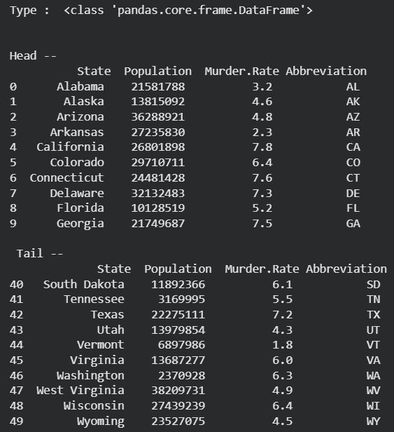
In this step we load a dataset using Pandas and explore its structure. We can check the type of data and print the first and last 10 records to get a idea of the dataset.

You can download dataset from here.

Python `

data = pd.read_csv("state.csv")

print ("Type : ", type(data), "\n\n")

print ("Head -- \n", data.head(10))

print ("\n Tail -- \n", data.tail(10))

`

**Output:

Output

Step 3: Adding and Modifying Columns

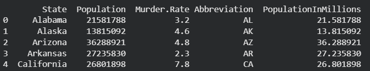
Derived columns are new columns created from existing ones. For example here we are converting the population into millions to make it more readable.

Python `

data['PopulationInMillions'] = data['Population']/1000000

print (data.head(5))

`

**Output:

Output

Sometimes, we may need to rename columns when column names contain special characters or spaces which cause issues in data manipulation. To do this we use .rename() function.

Python `

data.rename(columns ={'Murder.Rate': 'MurderRate'}, inplace = True) list(data)

`

**Output:

['State', 'Population', 'MurderRate', 'Abbreviation', 'PopulationInMillions']

Step 4: Describing the Data

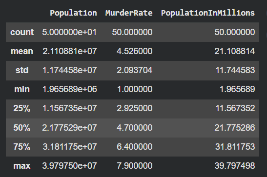
Using describe() provides a summary of the dataset which includes count, mean, standard deviation and more for each numerical column.

Python `

data.describe()

`

**Output:

Output

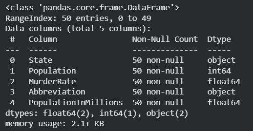
The info() method in pandas provides a summary of the dataset includes number of rows , column names, data types of each column and the memory usage of the entire dataframe. It helps to quickly understand the structure and size of the dataset.

Python `

data.info()

`

**Output:

Output

Step 5: Calculating Central Tendencies

Understanding the central tendencies of our data helps us summarize it effectively. In this step we will calculate different central tendency measures such as the mean, trimmed mean, weighted mean and median for the dataset's numerical columns.

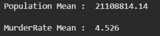
**1. Mean

The mean is the average value of a dataset. It's calculated by summing all values and dividing by the number of values. In pandas it can be with help of **mean() function.

Python `

Population_mean = data.Population.mean() print ("Population Mean : ", Population_mean)

MurderRate_mean = data.MurderRate.mean() print ("\nMurderRate Mean : ", MurderRate_mean)

`

**Output:

Output

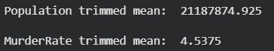
2. Trimmed Mean

Trimmed mean calculates the average by removing a certain percentage of the highest and lowest values in the dataset. This helps reduce the impact of outliers or extreme values that could skew the overall mean.

Python `

population_TM = trim_mean(data.Population, 0.1) print ("Population trimmed mean: ", population_TM)

murder_TM = trim_mean(data.MurderRate, 0.1) print ("\nMurderRate trimmed mean: ", murder_TM)

`

**Output:

Output

3. Weighted Mean

A weighted mean assigns different weights to different data points. Here we calculate the murder rate weighted by the population meaning larger states have more influence on the mean.

Python `

murderRate_WM = np.average(data.MurderRate, weights = data.Population) print ("Weighted MurderRate Mean: ", murderRate_WM)

`

**Output:

Weighted MurderRate Mean: 4.716864961131351

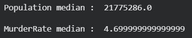
4. Median

The median is the middle value when the data is sorted and it is useful for understanding the central tendency especially when the data has outliers.

Python `

Population_median = data.Population.median() print ("Population median : ", Population_median)

MurderRate_median = data.MurderRate.median() print ("\nMurderRate median : ", MurderRate_median)

`

**Output:

Output

Here we have learn how to use Pandas to perform various EDA tasks such as loading data, inspecting data types, adding and modifying columns and calculating key statistics like mean, median and trimmed mean.