Python OpenCV Morphological Operations (original) (raw)

Morphological operations are image processing techniques used to modify the shape and structure of objects in an image. In OpenCV, these operations are typically applied to binary images using a kernel and are widely used for tasks such as noise removal, object enhancement, and boundary extraction.

**Shape-Based Processing: Operates on object geometry rather than individual pixel values.
**Feature Refinement: Enhances object boundaries and improves image quality for further analysis.

**Prerequisites

Morphological operations require:

**Binary Image: Contains foreground and background regions.
**Kernel (Structuring Element): Defines how neighboring pixels are processed.

Types of Morphological Operations

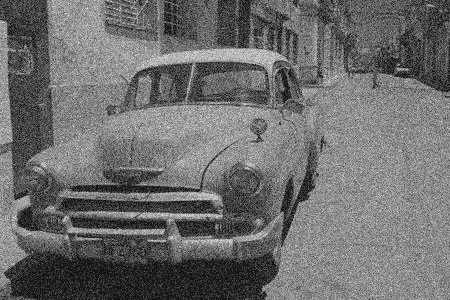
**Images used for demonstration:

Screenshot20220304172134-660x558

noise_car

**1. Erosion

Erosion shrinks the white foreground regions in a binary image. It removes small noise and makes object boundaries thinner by eliminating pixels from the edges of foreground objects.

**Code Implementation:

Convert the grayscale image into a binary image using Otsu's thresholding.
Create a 5 × 5 kernel and apply cv2.erode() to shrink foreground regions. Python `

import cv2, numpy as np, matplotlib.pyplot as plt img = cv2.imread(r"Downloads\test (2).png", 0) bin = cv2.threshold(img, 0, 255, cv2.THRESH_BINARY+cv2.THRESH_OTSU)[1]

k = np.ones((5, 5), np.uint8)
inv = cv2.bitwise_not(bin)
out = cv2.erode(inv, k, 1)
plt.imshow(out, cmap='gray'), plt.axis('off'), plt.show()

**Output:

The output image appears thinner than the original because pixels along the object boundaries are removed.

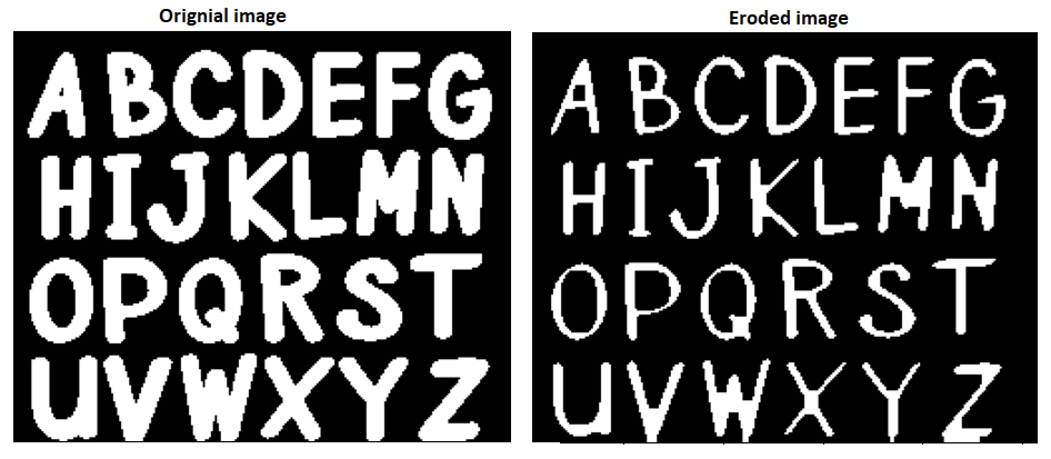
Erosion

2. Dilation

Dilation is a morphological operation that expands the white foreground regions in a binary image. It thickens object boundaries and fills small gaps by adding pixels to the edges of foreground objects.

**Code Implementation:

Convert the grayscale image into a binary image using Otsu's thresholding.
Create a 3 × 3 kernel and apply cv2.dilate() to expand foreground regions and connect nearby objects. Python `

import cv2, numpy as np, matplotlib.pyplot as plt

img = cv2.imread(r"Downloads\test (2).png", 0)
bin = cv2.threshold(img, 0, 255, cv2.THRESH_BINARY+cv2.THRESH_OTSU)[1]

k = np.ones((3, 3), np.uint8) inv = cv2.bitwise_not(bin)
out = cv2.dilate(inv, k, 1)
plt.imshow(out, cmap='gray'), plt.axis('off'), plt.show()

**Output:

The output image appears thicker than the original because pixels are added along the object boundaries.

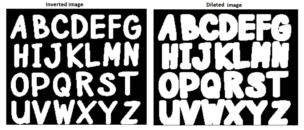
Dilated image

**3. Opening

Opening performs erosion followed by dilation on a binary image. It is commonly used to remove small noise and unwanted foreground objects while preserving the overall shape of larger objects.

**Code Implementation:

Create a 3 × 3 kernel to define the neighborhood used for the morphological operation.
Apply cv2.MORPH_OPEN to perform erosion followed by dilation, removing small foreground noise while preserving larger objects. Python `

import cv2, numpy as np, matplotlib.pyplot as plt

img = cv2.imread(r"Downloads\test (2).png", 0)
bin = cv2.threshold(img, 0, 255, cv2.THRESH_BINARY+cv2.THRESH_OTSU)[1]

k = np.ones((3, 3), np.uint8)
opened = cv2.morphologyEx(bin, cv2.MORPH_OPEN, k) plt.imshow(opened, cmap='gray'), plt.axis('off'), plt.show()

**Output:

The output image contains fewer small foreground noise regions while retaining the main object structures.

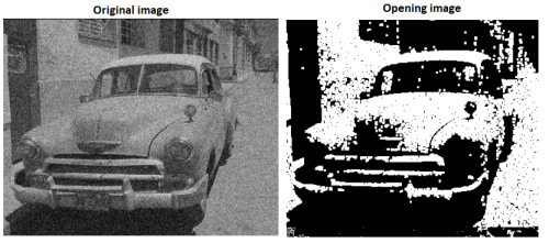
Opening Image

4. Closing

Closing performs dilation followed by erosion on a binary image. It is commonly used to fill small holes, connect nearby objects, and smooth object boundaries while preserving the overall shape of foreground regions.

**Code Implementation:

Create a 3 × 3 kernel to define the neighborhood used for the morphological operation.
Apply cv2.MORPH_CLOSE to perform dilation followed by erosion, filling small gaps and holes in foreground objects. Python `

import cv2, numpy as np, matplotlib.pyplot as plt

img = cv2.imread(r"Downloads\test (2).png", 0) bin = cv2.threshold(img, 0, 255, cv2.THRESH_BINARY+cv2.THRESH_OTSU)[1]

k = np.ones((3, 3), np.uint8) closed = cv2.morphologyEx(bin, cv2.MORPH_CLOSE, k)
plt.imshow(closed, cmap='gray'), plt.axis('off'), plt.show()

**Output:

The output image has small holes and gaps filled, resulting in smoother and more connected foreground objects.

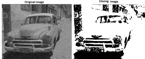
Closing Image

5. Morphological Gradient

Morphological Gradient highlights the boundaries of foreground objects by calculating the difference between the dilated and eroded versions of an image. It is commonly used for edge and boundary detection.

**Code Implementation:

Create a 3 × 3 kernel to define the neighborhood used for processing.
Apply cv2.MORPH_GRADIENT to extract the boundaries of foreground objects. Python `

import cv2, numpy as np, matplotlib.pyplot as plt img = cv2.imread(r"path to your image", 0)
bin = cv2.threshold(img, 0, 255, cv2.THRESH_BINARY+cv2.THRESH_OTSU)[1]

k = np.ones((3, 3), np.uint8)
inv = cv2.bitwise_not(bin)
out = cv2.morphologyEx(inv, cv2.MORPH_GRADIENT, k) plt.imshow(out, cmap='gray'), plt.axis('off'), plt.show()

**Output:

The output image displays the outlines of foreground objects, making their boundaries more prominent.

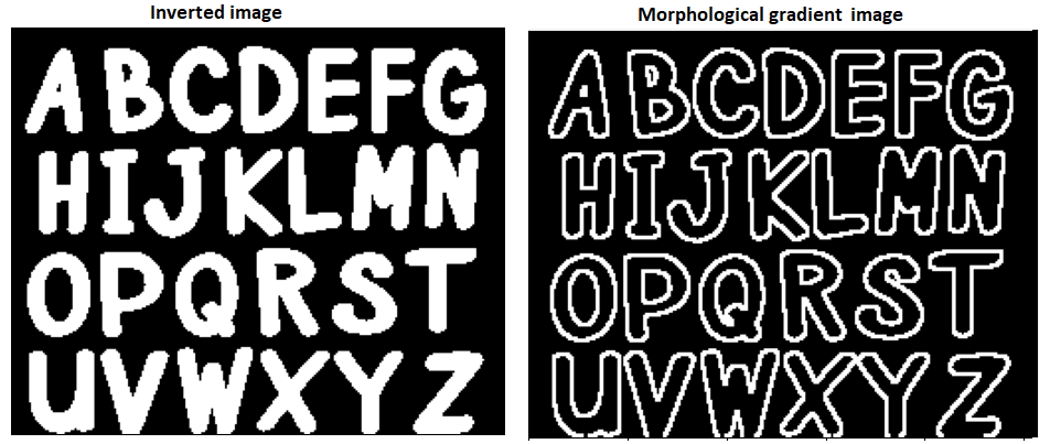
Morphological gradient Image

6. Top Hat

Top Hat extracts small bright regions from an image by calculating the difference between the original image and its opened version. It is commonly used to highlight fine details and bright objects that are smaller than the structuring element.

**Code Implementation:

Create a 13 × 13 kernel to define the structuring element used for the opening operation.
Apply cv2.MORPH_TOPHAT to extract bright regions that are removed during opening. Python `

import cv2, numpy as np, matplotlib.pyplot as plt img = cv2.imread("path", 0)

bin = cv2.threshold(img, 0, 255, cv2.THRESH_BINARY + cv2.THRESH_OTSU)[1] k = np.ones((13, 13), np.uint8) top = cv2.morphologyEx(bin, cv2.MORPH_TOPHAT, k) plt.imshow(top, cmap='gray'), plt.axis('off'), plt.show()

**Output:

The output image highlights small bright features while suppressing larger background regions.

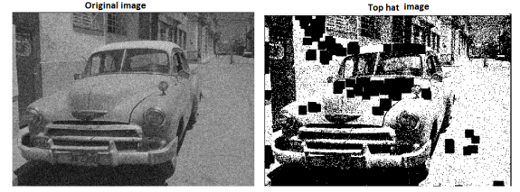
Top hat Image

7. Black Hat

Black Hat highlights small dark regions in an image by calculating the difference between the closed image and the original image. It is commonly used to enhance dark features that appear on a brighter background.

**Code Implementation:

Create a 5 × 5 kernel to define the structuring element used for the closing operation.
Apply cv2.MORPH_BLACKHAT to extract dark regions that are removed during closing. Python `

import cv2, numpy as np, matplotlib.pyplot as plt img = cv2.imread("path", 0)

bin = cv2.threshold(img, 0, 255, cv2.THRESH_BINARY + cv2.THRESH_OTSU)[1] inv = cv2.bitwise_not(bin) k = np.ones((5, 5), np.uint8) bh = cv2.morphologyEx(inv, cv2.MORPH_BLACKHAT, k) plt.imshow(bh, cmap='gray'), plt.axis('off'), plt.show()

**Output:

The output image highlights small dark features while suppressing the surrounding bright regions.

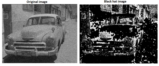
Black Hat image

You can download the source code from here.