SciPy Interpolation (original) (raw)
In this article, we will learn Interpolation using the SciPy module in Python. First, we will discuss interpolation and its types with implementation.
Interpolation and Its Types
Interpolation is a technique of constructing data points between given data points. The **scipy.interpolate is a module in Python SciPy consisting of classes, spline functions, and univariate and multivariate interpolation classes. Interpolation is done in many ways some of them are :
- 1-D Interpolation
- Spline Interpolation
- Univariate Spline Interpolation
- RBF Interpolation
Let's discuss all the methods one by one and visualize the results.
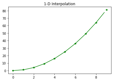
1-D Interpolation
To create a function based on fixed data points, **scipy.interpolate.interp1d is used. It takes data points x and y and returns a function that can be called with new x and returns the corresponding y point.
**Syntax: scipy.interpolate.interp1d(x , y , kind , axis , copy , bounds_error , fill_value , assume_sorted)
Python `
Import the required Python libraries
import matplotlib.pyplot as plt from scipy import interpolate import numpy as np
Initialize input values x and y
x = np.arange(0, 10) y = x**2
Interpolation
temp = interpolate.interp1d(x, y) xnew = np.arange(0, 9, 0.2) ynew = temp(xnew)
plt.title("1-D Interpolation") plt.plot(x, y, '*', xnew, ynew, '-', color="green") plt.show()
`
**Output:
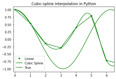
Spline Interpolation
In spline interpolation, a spline representation of the curve is computed, and then the spline is computed at the desired points. The function **splrep is used to find the spline representation of a curve in a two-dimensional plane.
**Note: As of SciPy version 1.15.1, scipy.interpolate.splrep is deprecated in favor of **scipy.interpolate.make_splrep. Although splrep is still functional, it is recommended to transition to make_splrep for better long-term support and future compatibility.
- To find the B-spline representation of a 1-D curve, **scipy.interpolate.make_splrep is used.
**Syntax: scipy.interpolate.make_splrep(x, y, w=None, xb=None, xe=None, k=3, s=None, full_output=0, per=0)
- To compute a B-spline or its derivatives, **scipy.interpolate.splev is used.
**Syntax: scipy.interpolate.splev(x , tck , der , ext)
Python `
Import the required Python libraries
import numpy as np import matplotlib.pyplot as plt from scipy import interpolate
Initialize the input values
x = np.arange(0, 10) y = np.cos(x**3)
Interpolation using make_splrep (updated)
To find the spline representation of a
curve in a 2-D plane using make_splrep
temp = interpolate.make_splrep(x, y, s=0) xnew = np.arange(0, np.pi**2, np.pi/100) ynew = interpolate.splev(xnew, temp, der=0)
plt.figure() plt.plot(x, y, '*', xnew, ynew, xnew, np.cos(xnew), x, y, 'b', color="green") plt.legend(['Linear', 'Cubic Spline', 'True']) plt.axis([-0.1, 6.5, -1.1, 1.1]) plt.title('Cubic-spline Interpolation in Python') plt.show()
`
**Output:
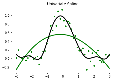
Univariate Spline
It is a 1-D smoothing spline that fits a given group of data points. The **scipy.interpolate.UnivariateSpline is used to fit a spline y = spl(x) of degree k to the provided x, y data. s specifies the number of knots by specifying a smoothing condition. The **scipy.interpolate.UnivariateSpline. set_smoothing_factor: Spline computation with the given smoothing factor s and with the knots found at the last call.
**Syntax: scipy.interpolate.UnivariateSpline( x, y, w, bbox, k, s, ext)
Python `
Import the required libraries
import matplotlib.pyplot as plt from scipy.interpolate import UnivariateSpline
x = np.linspace(-3, 3, 50) y = np.exp(-x**2) + 0.1 * np.random.randn(50) plt.title("Univariate Spline") plt.plot(x, y, 'g.', ms=8)
Using the default values for the
smoothing parameter
spl = UnivariateSpline(x, y) xs = np.linspace(-3, 3, 1000) plt.plot(xs, spl(xs), 'green', lw=3)
Manually change the amount of smoothing
spl.set_smoothing_factor(0.5) plt.plot(xs, spl(xs), color='black', lw=3) plt.show()
`
**Output:
Radial basis function for Interpolation
The scipy.interpolate.Rbf is used for interpolating scattered data in n-dimensions. The radial basis function is defined as corresponding to a fixed reference data point. The scipy.interpolate.Rbf is a class for radial basis function interpolation of functions from N-D scattered data to an M-D domain.
**Syntax: scipy.interpolate.Rbf(*args)
Python `
Import the required libraries
import numpy as np from scipy.interpolate import Rbf import matplotlib.pyplot as plt
setup the data values
x = np.linspace(0, 10, 9) y = np.cos(x/2) xi = np.linspace(0, 10, 110)
Interpolation using RBF
rbf = Rbf(x, y) fi = rbf(xi)
plt.subplot(2, 1, 2) plt.plot(x, y, '*', color="green") plt.plot(xi, fi, 'green') plt.plot(xi, np.sin(xi), 'black') plt.title('Radial basis function Interpolation') plt.show()
`