scipy stats.halflogistic() | Python (original) (raw)
Last Updated : 27 Mar, 2019
scipy.stats.halflogistic() is an Half-logistic continuous random variable that is defined with a standard format and some shape parameters to complete its specification.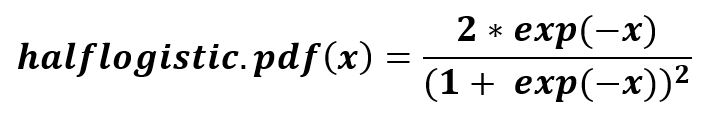
Parameters : -> q : lower and upper tail probability-> x : quantiles-> loc : [optional]location parameter. Default = 0-> scale : [optional]scale parameter. Default = 1-> size : [tuple of ints, optional] shape or random variates.-> moments : [optional] composed of letters [‘mvsk’]; 'm' = mean, 'v' = variance, 's' = Fisher's skew and 'k' = Fisher's kurtosis. (default = 'mv'). Results : Half-logistic continuous random variable
Code #1 : Creating Half-logistic continuous random variable
Python3 `
from scipy.stats import halflogistic
numargs = halflogistic .numargs [] = [0.7, ] * numargs rv = halflogistic ()
print ("RV : \n", rv)
`
Output :
RV : <scipy.stats._distn_infrastructure.rv_frozen object at 0x000001E39A2EA7B8>
Code #2 : Half-logistic random variates and probability distribution
Python3 `
import numpy as np quantile = np.arange (0.01, 1, 0.1)
Random Variates
R = halflogistic .rvs(scale = 2, size = 10) print ("Random Variates : \n", R)
R = halflogistic .pdf(quantile, loc = 0, scale = 1) print ("\nProbability Distribution : \n", R)
`
Output :
Random Variates : [1.51677656 4.2051329 3.00947016 5.00828865 8.23514322 0.46379571 1.75794767 2.84948119 0.31392647 1.36186056]
Probability Distribution : [0.4999875 0.49849054 0.49452777 0.48817731 0.47956248 0.46884669 0.45622704 0.44192689 0.42618788 0.40926186]
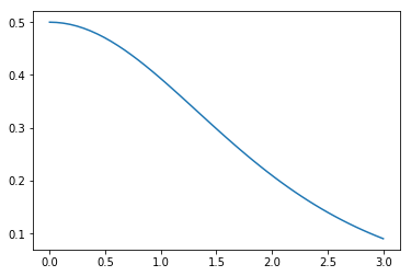
Code #3 : Graphical Representation.
Python3 `
import numpy as np import matplotlib.pyplot as plt
distribution = np.linspace(0, np.minimum(rv.dist.b, 3)) print("Distribution : \n", distribution)
plot = plt.plot(distribution, rv.pdf(distribution))
`
Output :
Distribution : [0. 0.06122449 0.12244898 0.18367347 0.24489796 0.30612245 0.36734694 0.42857143 0.48979592 0.55102041 0.6122449 0.67346939 0.73469388 0.79591837 0.85714286 0.91836735 0.97959184 1.04081633 1.10204082 1.16326531 1.2244898 1.28571429 1.34693878 1.40816327 1.46938776 1.53061224 1.59183673 1.65306122 1.71428571 1.7755102 1.83673469 1.89795918 1.95918367 2.02040816 2.08163265 2.14285714 2.20408163 2.26530612 2.32653061 2.3877551 2.44897959 2.51020408 2.57142857 2.63265306 2.69387755 2.75510204 2.81632653 2.87755102 2.93877551 3. ]
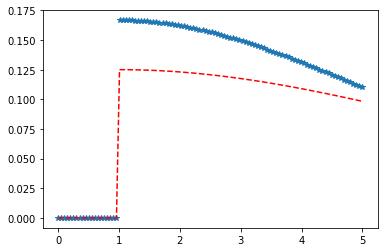
 Code #4 : Varying Positional Arguments
Python3 `
import matplotlib.pyplot as plt import numpy as np
x = np.linspace(0, 5, 100)
Varying positional arguments
y1 = halflogistic .pdf(x, 1, 3) y2 = halflogistic .pdf(x, 1, 4) plt.plot(x, y1, "*", x, y2, "r--")
`
Output :