Solve Differential Equations with ODEINT Function of SciPy module in Python (original) (raw)

Last Updated : 7 Jul, 2025

In science and engineering, many problems involve quantities that change over time like speed of a moving object or temperature of a cooling cup. These changes are often described using differential equations.

SciPy provides a function called odeint (from the scipy.integrate module) that helps solve these equations numerically. By giving it a function that describes how your system changes and some starting values, odeint calculates how the system behaves over time.

Syntax

scipy.integrate.odeint (func, y0, t, args=())

**Parameter:

• **func: function that returns the derivative (dy/dt).
• **y 0 : initial conditions.
• **t: time points to solve the ODE at.
• **args (optional): extra values passed to func.

Solving Differential Equations

Let's solve an ordinary differential equation (ODE) using the **odeint() function.

Example 1

\frac{dy}{dt} = -yt + 13

Python `

import numpy as np from scipy.integrate import odeint import matplotlib.pyplot as plt

Initial condition

y0 = 1

Time points

t = np.linspace(0, 5)

Define the differential equation using lambda

dy/dt = -y * t + 13

dydt = lambda y, t: -y * t + 13

Solve the ODE

y = odeint(dydt, y0, t)

plt.plot(t, y) plt.xlabel("Time") plt.ylabel("Y") plt.show()

`

**Output

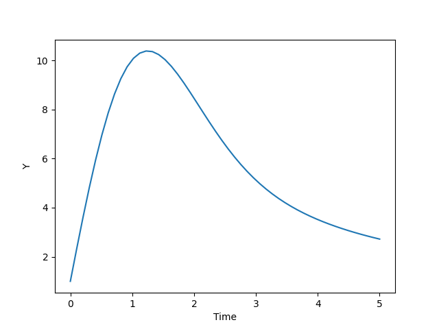
Graph for the solution of ODE

**Explanation:

• Defines and solves the ODE dy/dt = -y * t + 13 using odeint with initial value y = 1.
• The graph shows how **y changes over time.
• y increases first then slows as -y * t term grows.

Example 2

\frac{dy}{dt} = 13e^t + y

Python `

import numpy as np from scipy.integrate import odeint import matplotlib.pyplot as plt

Initial condition

y0 = 1

Time values

t = np.linspace(0, 5)

Define ODE directly using lambda: dy/dt = 13 * e^t + y

dydt = lambda y, t: 13 * np.exp(t) + y

Solve ODE

y = odeint(dydt, y0, t)

plt.plot(t, y) plt.xlabel("Time") plt.ylabel("Y") plt.show()

`

**Output

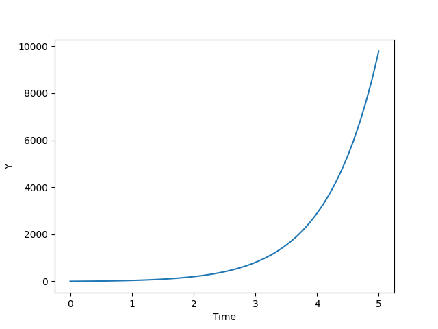
Graph for the solution of ODE

**Explanation:

• Defines and solves ODE dy/dt = 13*eᵗ + y using odeint starting from y = 1.
• The graph shows y grows rapidly, driven by both exponential and linear terms.
• The exponential term accelerates the growth of y as time increases.

Example 3

\frac{dy}{dt} = \frac{1 - y}{1.95 - y} - \frac{y}{0.05 + y}

Python `

import numpy as np from scipy.integrate import odeint import matplotlib.pyplot as plt

Initial conditions

y0 = [0, 1, 2]

Time values

t = np.linspace(1, 10)

Define the ODE using lambda

dydt = lambda y, t: (1 - y) / (1.95 - y) - y / (0.05 + y)

Solve the ODE

y = odeint(dydt, y0, t)

plt.plot(t, y) plt.xlabel("Time") plt.ylabel("Y") plt.show()

`