Benford's Distribution in R (original) (raw)

Last Updated : 23 Jul, 2025

Benford's Law, also known as the **First-Digit Law or **Benford's Distribution, is a fascinating statistical phenomenon that predicts the frequency of the first digits in many real-life datasets. Unlike what one might expect (i.e., an equal probability for all digits from 1 to 9), Benford's law states that lower digits appear more frequently than the first digit.

**What is Benford's Law?

Benford's Distribution has significant applications in fraud detection, forensic accounting, and data validation. This article explores Benford's Law, its mathematical basis, practical applications, and how to apply and visualize it using R. Benford's Law states that in many naturally occurring datasets, the leading digit d (where d ranges from 1 to 9) occurs with a probability given by:

P(d) = \log_{10}\left(1 + \frac{1}{d}\right)

**Applications of Benford's Law

Benford's Law is widely used in:

• **Fraud Detection: Detecting anomalies in financial statements, tax records, or election data.
• **Auditing: Ensuring data integrity and validating datasets.
• **Data Science: Identifying inconsistencies in data reporting or collection.

Now we will discuss step by step implementation of Benford's Distribution in R Programming Language.

**Step 1: Install and Load Required Packages

To analyze Benford's Distribution, we will use the benford.analysis package. This package provides easy-to-use functions to analyze and visualize data according to Benford's Law.

R `

Install the benford.analysis package

if (!require(benford.analysis)) install.packages("benford.analysis", dependencies = TRUE) library(benford.analysis)

`

**Step 2: Prepare Your Data

Before applying Benford's Law, ensure your dataset is suitable:

• Data should be positive, real numbers.
• The dataset should ideally span multiple orders of magnitude.

For demonstration, let's create a simple dataset that spans multiple orders of magnitude.

R `

Create a sample dataset

set.seed(123) sample_data <- c(1000 * runif(1000), 10000 * runif(1000), 100000 * runif(1000))

`

**Step 3: Applying Benford's Analysis

The benford() function in the benford.analysis package can be used to apply Benford's analysis on your dataset.

R `

Apply Benford's analysis on the sample dataset

benford_result <- benford(sample_data, number.of.digits = 1)

Display the summary of the analysis

summary(benford_result)

`

**Output:

              Length Class      Mode       

info 4 -none- list
data 4 data.table list
s.o.data 2 data.table list
bfd 13 data.table list
mantissa 2 data.table list
MAD 1 -none- numeric
MAD.conformity 1 -none- character
distortion.factor 1 -none- numeric
stats 2 -none- list

**Step 4: Visualizing Benford's Distribution

Visualization is a crucial step to understand how closely your data follows Benford's Law. The plot() function in the benford.analysis package allows you to generate multiple visualizations.

R `

Plot the Benford analysis result

plot(benford_result)

`

**Output:

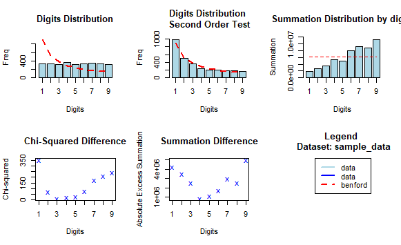
Benford's Distribution in R

This function generates a bar plot comparing the actual frequency of the leading digits in your dataset against the expected frequencies according to Benford's Law.

**Step 5: Evaluating the Performance

You can perform additional tests to check how well your data fits Benford's Law:

• **MAD (Mean Absolute Deviation): Measures how much the observed distribution deviates from Benford’s Law.
• **Chi-Square Test: A statistical test to determine if your data significantly deviates from Benford's Law. R `

Perform a Chi-Square goodness-of-fit test

chi_square_result <- chisq(benford_result) print(chi_square_result)

`

**Output:

Pearson's Chi-squared test

data: sample_data
X-squared = 1186.6, df = 8, p-value < 2.2e-16

A non-significant result (high p-value) indicates that the dataset follows Benford's Law closely.

**Practical Considerations and Limitations

• **Data Characteristics: Not all datasets follow Benford's Law. It works best with datasets that span multiple orders of magnitude and where numbers arise from natural or human processes.
• **Sample Size: Small datasets may not provide reliable results. A larger sample size generally leads to more accurate analysis.
• **Non-Suitability: Datasets with assigned or regulated numbers (telephone numbers, ZIP codes) don't follow Benford’s Law.

**Conclusion

Benford's Law is a powerful tool in the world of statistics and data analysis, providing insights into data authenticity and helping to detect irregularities. In R, the benford.analysis package offers an easy and efficient way to analyze datasets according to Benford's Law, complete with statistical tests and visualizations. By understanding how to apply Benford's Distribution in R, you can use this technique to uncover anomalies in datasets, making it particularly useful in fraud detection, auditing, and other fields where data integrity is crucial.