Binomial Distribution in R Programming (original) (raw)

Last Updated : 12 Jul, 2025

Binomial distribution in R is a probability distribution used in statistics. The binomial distribution is a discrete distribution and has only two outcomes i.e. success or failure. All its trials are independent, the probability of success remains the same and the previous outcome does not affect the next outcome. The outcomes from different trials are independent. Binomial distribution helps us to find the individual probabilities as well as cumulative probabilities over a certain range.

It is also used in many real-life scenarios such as in determining whether a particular lottery ticket has won or not, whether a drug is able to cure a person or not, it can be used to determine the number of heads or tails in a finite number of tosses, for analyzing the outcome of a die, etc.

Formula

P(X = k) = \binom{n}{k} p^k (1 - p)^{n - k}

Where:

**P(X=k): Represents the probability of getting exactly **k successes.
\binom{n}{k}: The binomial coefficient, also known as "n choose k", calculates the number of ways to choose **k successes from **n trials.
pk: The probability of success raised to the power of **k.
(1 - p)^{n - k}: The probability of failure raised to the power of the remaining trials.

Functions for Binomial Distribution

We have four functions for handling binomial distribution in R namely:

dbinom()
pbinom()
qbinom()
rbinom()

dbinom() Function

This function is used to find probability at a particular value for a data that follows binomial distribution i.e. it finds:

P(X = k)

**Syntax:

dbinom(k, n, p)

**Example:

Python `

dbinom(3, size = 13, prob = 1 / 6) probabilities <- dbinom(x = c(0:10), size = 10, prob = 1 / 6) data.frame(x, probs) plot(0:10, probabilities, type = "l")

**Output :

dbinom(3, size = 13, prob = 1/6)
[1] 0.2138454
probabilities = dbinom(x = c(0:10), size = 10, prob = 1/6)
data.frame(probabilities)
probabilities
1 1.615056e-01
2 3.230112e-01
3 2.907100e-01
4 1.550454e-01
5 5.426588e-02
6 1.302381e-02
7 2.170635e-03
8 2.480726e-04
9 1.860544e-05
10 8.269086e-07
11 1.653817e-08

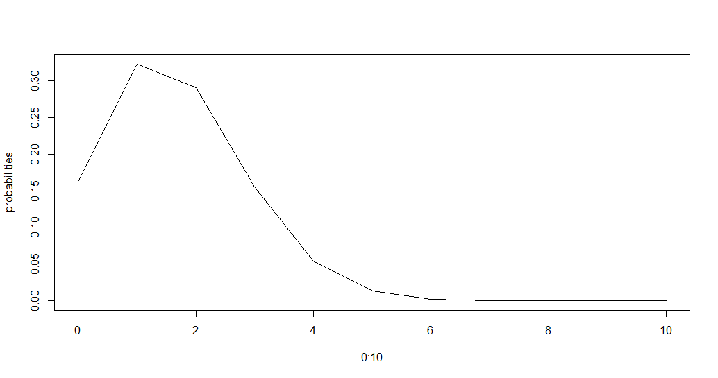
**Explanation: The above piece of code first finds the probability at k=3, then it displays a data frame containing the probability distribution for k from 0 to 10 which in this case is 0 to n.

pbinom()Function

The function pbinom() is used to find the cumulative probability of a data following binomial distribution till a given value ie it finds:

P(X <= k)

**Syntax:

pbinom(k, n, p)

**Example:

Python `

pbinom(3, size = 13, prob = 1 / 6) plot(0:10, pbinom(0:10, size = 10, prob = 1 / 6), type = "l")

**Output :

pbinom(3, size = 13, prob = 1/6)
[1] 0.8419226

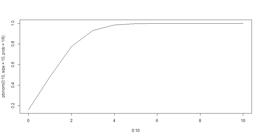
**Explanation: The code calculates and plots the cumulative binomial distribution for a given number of trials and success probability. pbinom() calculates the cumulative probability, and plot() visualizes it.

qbinom() Function

This function is used to find the nth quantile, that is if P(x <= k) is given, it finds k.

**Syntax:

qbinom(P, n, p)

**Example:

Python `

qbinom(0.8419226, size = 13, prob = 1 / 6) x <- seq(0, 1, by = 0.1) y <- qbinom(x, size = 13, prob = 1 / 6) plot(x, y, type = 'l')

**Output :

qbinom(0.8419226, size = 13, prob = 1/6)
[1] 3

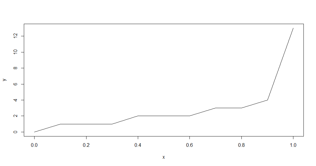
**Explanation: This R code calculates the binomial quantile for a given probability and plots the binomial quantiles against cumulative probabilities.

rbinom() Function

This function generates n random variables of a particular probability.

**Syntax:

rbinom(n, N, p)

**Example:

Python `

rbinom(8, size = 13, prob = 1 / 6) hist(rbinom(8, size = 13, prob = 1 / 6))

**Output:

rbinom(8, size = 13, prob = 1/6)
[1] 1 1 2 1 4 0 2 3

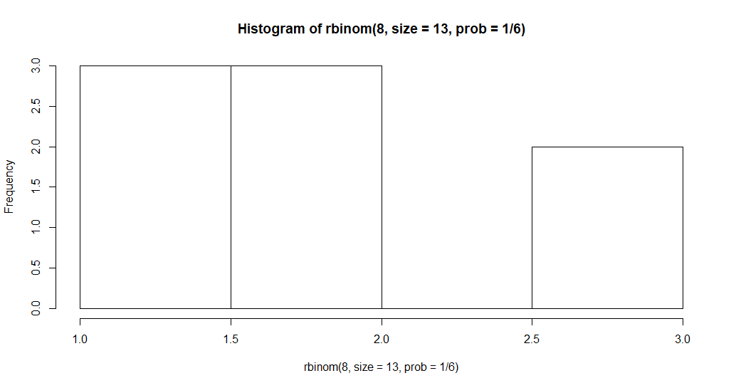
**Explanation: This R code generates 8 random samples from a binomial distribution and creates a histogram to visualize the distribution of those samples.