Decision Tree for Regression in R Programming (original) (raw)

Last Updated : 15 Jul, 2025

A decision tree is a machine learning algorithm used to predict continuous values (regression) or categories (classification). In regression, a decision tree is used when the dependent variable is continuous, like predicting car mileage based on engine power.

Working of Decision Tree Algorithm of Regression

A decision tree for regression works by recursively partitioning the dataset into subsets based on feature values. The goal is to minimize the variance of the target variable (dependent variable) within each subset.

1. **Splitting the Data

At each node, the decision tree selects the feature X_j​ and a split point s_j​ such that the sum of variances within the resulting subsets is minimized. The **variance of the target variable Y within a subset is calculated as:

\text{Var}(Y|X_j, s_j) = \frac{1}{N} \sum_{i=1}^{N} (y_i - \bar{y})^2

Where:

• y_i​ is the actual target value of the i^{th} sample,
• \bar{y}​ is the mean of yvalues in that subset,
• N is the number of samples in the subset.

The split at each node aims to find the feature X_j​ and threshold s_j​ that minimize the **total variance across the two child nodes:

\text{Total Variance} = \frac{N_L}{N} \text{Var}(Y|X_j, s_j)_L + \frac{N_R}{N} \text{Var}(Y|X_j, s_j)_R

Where:

• N_L and N_R​ are the number of samples in the left and right child nodes,
• \text{Var}(Y|X_j, s_j)_L and \text{Var}(Y|X_j, s_j)_R​ are the variances in the left and right child nodes.

2. **Leaf Node Prediction

Once the data is split sufficiently, each leaf node will contain a subset of the data, and the prediction for that subset is the **mean value of the target variable Y:

​\hat{y} = \frac{1}{N_{\text{leaf}}} \sum_{i=1}^{N_{\text{leaf}}} y_i

Where:

• \hat{y} is the predicted value for all data points in that leaf,
• N_{\text{leaf}} is the number of samples in that leaf.

3. **Making Predictions

To predict a new data point \mathbf{x}, the decision tree follows the splits starting from the root to the appropriate leaf node. Once in the leaf node, the prediction is the mean of the target values in that node:

\hat{y}_{\text{new}} = \frac{1}{N_{\text{leaf}}} \sum_{i=1}^{N_{\text{leaf}}} y_i

Where:

• N_{\text{leaf}} is the number of samples in the leaf that the new data point \mathbf{x} falls into.

Implementation of Decision Tree for Regression in R

We will now demonstrate how to predict the mpg (miles per gallon) using a regression decision tree.

1. Installing and loading the Required Package

We will install the **rpart package, which contains the necessary functions for decision tree regression.

R `

install.packages("rpart") library(rpart)

`

2. Loading the Dataset

We will load the **mtcars dataset, which is an in-built dataset in R. We will also use head() function to display first few rows.

R `

data(mtcars) head(mtcars)

`

**Output:

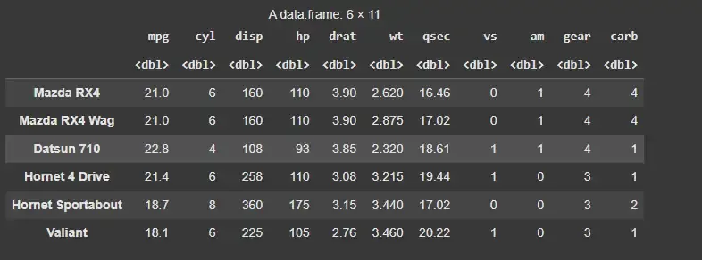
mtcars dataset

3. Fitting the Model

We will create a regression decision tree to predict mpg based on disp, hp, and cyl using the **rpart() function.

• **mpg ~ disp + hp + cyl: This specifies the formula where mpg is the dependent variable, and disp, hp, and cyl are the independent variables.
• **method = "anova": This specifies that we are performing regression, where the algorithm minimizes variance to predict continuous values.
• **data = mtcars: This specifies the dataset to be used for building the model, in this case, the mtcars dataset. R `

fit <- rpart(mpg ~ disp + hp + cyl, method = "anova", data = mtcars)

`

4. Plotting the Decision Tree

We will visualize the decision tree by plotting it and saving it as a PNG image.

• **png(): Opens a PNG device to save the plot to a file.
• **plot(): Creates a visual representation of the decision tree.
• **text(): Adds text labels to the plot, showing details like the number of observations at each node.
• **dev.off(): Closes the plotting device, saving the image. R `

png(file = "decTree2GFG.png", width = 600, height = 600) plot(fit, uniform = TRUE, main = "MPG Decision Tree using Regression") text(fit, use.n = TRUE, cex = .9) dev.off()

`

**Output:

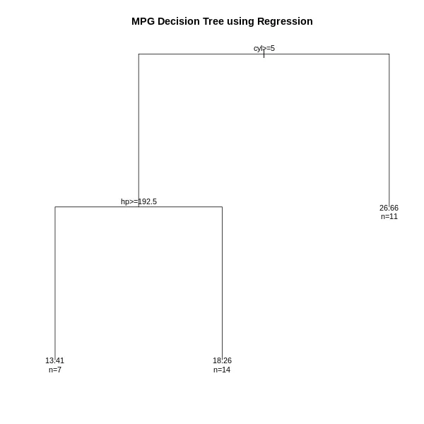
Decision Tree Structure

5. Printing the Decision Tree Model

We will print the decision tree model to view the splits and other details.

• **print(fit): Displays the decision tree structure, showing how the data was split at each node, the resulting outcomes, and the final predictions. R `

print(fit)

`

**Output:

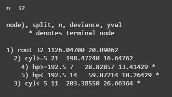
Decision Tree Model

6. Predicting MPG with Test Data

We will create a test dataset and use the decision tree model to predict the mpg value for a new set of inputs.

• **df: A new dataset containing the input values for which we want to predict mpg.
• **predict(): Uses the trained model (fit) to predict the mpg value for the new data.
• **method = "anova": Specifies that we are using regression to predict continuous values. R `

df <- data.frame(disp = 351, hp = 250, cyl = 8) cat("Predicted value:\n") predict(fit, df, method = "anova")

`

**Output:

Predicted value:
13.41429

Advantages of Decision Trees

• **Consider All Possible Decisions: Decision trees evaluate all potential decisions and create a comprehensive model for predictions.
• **Easy to Use: Simple to implement and interpret for both classification and regression tasks.
• **Handles Missing Values: Decision trees can manage datasets with missing values without requiring special preprocessing.

Disadvantages of Decision Trees

• **Computationally Intensive: For large datasets, decision trees can be slow to compute.
• **Limited Learning Capability: Decision trees may not perform well with complex data. Techniques like Random Forests can be used for improved performance.