Encoding Categorical Data in R (original) (raw)

Last Updated : 12 Mar, 2026

Encoding is the process of converting categorical data into numerical values. Categorical data is a type of data which can be classified into categories or groups (such as colors or job titles). Since categorical variables cannot be directly used in statistical analysis or machine learning models, encoding is necessary to represent them in a format that models can process.

• Encoding allows machine learning algorithms to interpret and learn from categorical variables effectively.
• Proper encoding helps prevent bias and ensures that model predictions are accurate.
• It enables seamless integration of categorical data in statistical analysis, visualization and modeling workflows.

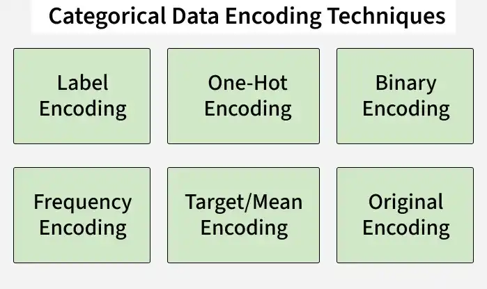
Encoding Techniques

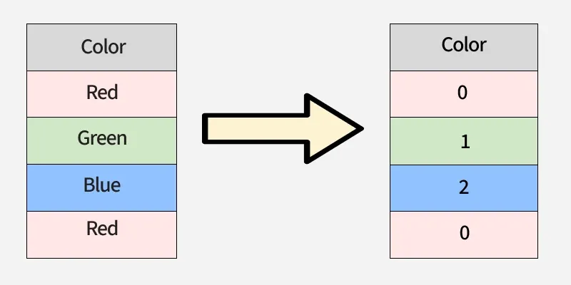
1. Label Encoding

Label Encoding is a technique that converts categorical variables into numeric values by assigning a unique integer to each category. In R, this can be done using the factor() function followed by as.integer() to get the numeric representation.

• Each category is assigned a distinct integer value, making it simple and memory-efficient.
• May unintentionally introduce an order among categories, which can affect models that assume numerical relationships.
• Commonly used in tree-based models like Decision Trees, Random Forests and XGBoost, which are not sensitive to the numeric order of labels.

Label Encoding

Here we implement Label Encoding in R for the ‘color’ column using factor() and as.integer() to convert each category into a unique numeric value.

• factor(df$color) converts the categorical column into a factor.
• as.integer() assigns each level of the factor a unique integer. R `

color <- c("red", "green", "blue", "blue", "red") df <- data.frame(color)

df$color <- as.integer(factor(df$color))

df

`

Output

color 1 3 2 2 3 1 4 1 5 3

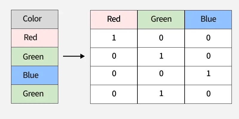
2. One-Hot Encoding

One-Hot Encoding is a technique used to convert categorical data into a binary format, where each unique category becomes its own column. This ensures that models can process categorical variables without assuming any order between categories.

• Each category is represented as a separate column, with 1 indicating presence and 0 indicating absence.
• Prevents false ordinal relationships, making it ideal for algorithms that assume numerical order such as linear models and neural networks
• Can increase dimensionality and produce sparse data when a feature has many unique categories.

One-Hot Encoding

Here we implement One-Hot Encoding in R for the ‘gender’ column using model.matrix() to convert categories into binary columns.

R `

gender <- c("male", "female", "male", "male", "female") age <- c(23, 34, 52, 21, 19) income <- c(50000, 70000, 80000, 45000, 55000) df <- data.frame(gender, age, income)

encoded_gender <- model.matrix(~ gender - 1, data = df)

encoded_gender

`

Output

genderfemale gendermale 1 0 1 2 1 0 3 0 1 4 0 1 5 1 0 attr(,"assign") [1] 1 1 attr(,"contrasts") a...

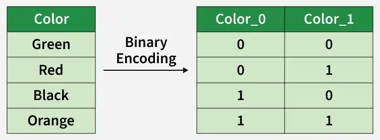
3. Binary Encoding

Binary Encoding is a method that converts categorical variables into binary numbers and splits these binary digits across multiple columns. It is especially useful for features with many unique categories because it reduces the number of columns compared to One-Hot Encoding.

• Each category is first converted to a numeric label, then represented in binary form across multiple columns.
• Efficient for high-cardinality categorical data, saving memory and reducing dimensionality.
• Commonly applied in text or NLP tasks where features have many unique values, but requires careful handling of missing data and slightly more complex implementation.

Binary Encoding

Here we implement Binary Encoding in R using the mltools package to convert the ‘color’ column into binary columns.

• The binary_encode() function converts each category into a binary code split across columns.
• Reduces the number of columns compared to One-Hot Encoding for features with many categories.
• Useful when working with models sensitive to high-dimensional sparse data. R `

city <- c("Delhi", "Mumbai", "Delhi", "Chennai", "Mumbai") df <- data.frame(City = city) df$Label <- as.numeric(factor(df$City)) - 1 decimal_to_binary <- function(x){ paste(rev(as.integer(intToBits(x))[1:4]), collapse = "") } df$Binary <- sapply(df$Label, decimal_to_binary)

print(df)

`

Output

 City Label Binary

1 Delhi 1 0001 2 Mumbai 2 0010 3 Delhi 1 0001 4 Chennai 0 0000 5 Mumbai 2 0010

4. Frequency Encoding

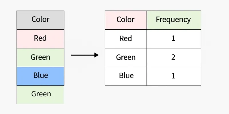
Frequency Encoding is a method that replaces each category with its occurrence frequency in the dataset. It provides a compact numerical representation of categorical data, making it suitable for datasets with many categories.

• Each category is assigned a value equal to the number of times it appears in the dataset.
• Efficient for large datasets and useful in domains like retail, e-commerce or clickstream analysis to capture popularity trends.
• While simple and memory-efficient, improper use can lead to data leakage if frequencies from the test set are mixed with the training set.

Frequency Encoding

Here we implement Frequency Encoding in R by replacing each category with its occurrence count in the dataset.

R `

color <- c("red", "green", "blue", "blue", "red", "red") df <- data.frame(color)

freq_table <- table(df$color) df$color_freq <- freq_table[df$color]

df

`

Output

color color_freq 1 red 3 2 green 1 3 blue 2 4 blue 2 5 red 3 6 red 3

5. Target/Mean Encoding

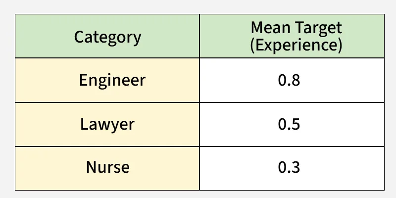
Target Encoding, also called Mean Encoding, replaces each category in a feature with the mean value of the target variable for that category. This allows models to capture the relationship between the categorical feature and the target.

• Each category is represented by the average value of the target variable for that category.
• Effective for high-cardinality features like ZIP codes, product IDs or user IDs.
• Can improve predictive power but may cause overfitting, so smoothing or cross-validation techniques are often used.

Target Encoding

Here we implement Target/Mean Encoding in R by replacing each category with the mean of the target variable for that category.

R `

df <- data.frame( product = c("A", "B", "A", "C", "B", "C", "A"), sales = c(200, 150, 220, 130, 160, 140, 210) ) mean_sales <- tapply(df$sales, df$product, mean) df$product_mean <- mean_sales[df$product]

df

`

Output

product sales product_mean 1 A 200 210 2 B 150 155 3 A 220 210 4 C 130 135 5 B 160 155 6 C 140 1...

6. Ordinal Encoding

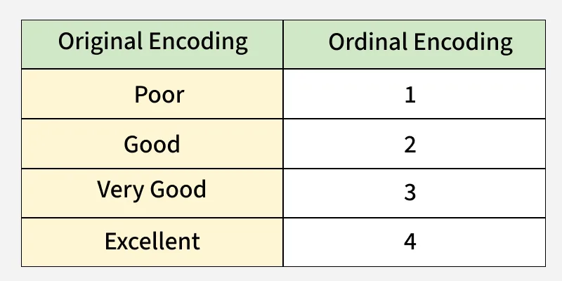
Ordinal Encoding is a method that assigns integer values to categories based on their natural order or ranking. Unlike Label Encoding, the order of categories is meaningful and preserved in the numeric representation.

• Categories are mapped to integers reflecting their order.
• Useful for features where a logical ranking exists, such as education level, customer satisfaction or rating scales.
• Improper use on nominal data can mislead models, so it should only be applied to ordinal variables.

Ordinal Encoding

Here we implement Ordinal Encoding in R by assigning integers to categories based on their natural order.

R `

education <- c("High School", "Bachelor", "Master", "Bachelor", "PhD") df <- data.frame(education) education_levels <- c("High School", "Bachelor", "Master", "PhD") df$education_encoded <- as.integer(factor(df$education, levels = education_levels, ordered = TRUE)) df

`

Output

education education_encoded

1 High School 1 2 Bachelor 2 3 Master 3 4 Bachelor 2 5 PhD 4