Exponential Smoothing in R Programming (original) (raw)
Last Updated : 14 Apr, 2026
Exponential Smoothing is a time series forecasting method that predicts future values by assigning exponentially decreasing weights to past observations. In this approach, recent data points have a greater influence on the forecast while the impact of older observations gradually decreases over time. In R programming, exponential smoothing can be used to analyze and forecast time series data such as sales trends, stock prices, demand patterns and production levels.
- Helps smooth short-term fluctuations in time series data, making underlying patterns easier to observe and interpret.
- Requires only a smoothing parameter and previous observations, which makes the method simple and efficient to implement in R.
- Useful for generating short-term forecasts in time series datasets where recent observations are more relevant than older data.
Here, we see different types of exponential smoothing techniques.
1. Simple Exponential Smoothing (SES)
Simple Exponential Smoothing (SES) is a forecasting method used for time series data that has no trend or seasonal pattern. It smooths the data by giving more weight to recent observations and less weight to older ones. The method uses a smoothing parameter \alpha(0–1) to control how quickly past values lose influence.
- A small \alpha gives more weight to past observations, resulting in smoother forecasts that react slowly to changes.
- A large \alpha gives more weight to recent observations, allowing the model to respond more quickly to new data.
Mathematical Representation of SES
s_t = s_{t-1} + \alpha (x_t - s_{t-1})
where
- s_{t}: smoothed value
- x_{t}: actual observation at time t
- s_{t-1}: previous smoothed value
- \alpha: smoothing parameter
- t: time period
Step By Step Implementation
Here we implement Simple Exponential Smoothing on the Google stock price dataset (goog). This technique is ideal for time series data without trend or seasonality, assigning more weight to recent observations for better short-term forecasting.
**Step 1: Installing and loading the required packages
We install the required packages using the install.packages() function.
- **fpp2: contains time series datasets and loads the forecast package.
- tidyverse: used for data manipulation and visualization. R `
install.packages("tidyverse") install.packages("fpp2")
`
**Step 2: Loading the required packages
We load the installed packages into the R environment using library() function.
R `
library(tidyverse) library(fpp2)
`
**Step 3: Splitting the dataset into training and testing sets
We split the Google stock data (goog) into a training set and a test set using window().
- **window(): extracts a specific time period from a time series object.
- **start: Specifies the time point to begin the subset (inclusive).
- **end: Specifies the time point to end the subset (inclusive). R `
goog.train <- window(goog, end = 900) goog.test <- window(goog, start = 901)
`
**Step 4: Performing SES on training data
We apply the ses() function with alpha = 0.2 and forecast horizon h = 100.
- **ses(): performs simple exponential smoothing.
- **alpha: smoothing constant controlling how much recent values influence the forecast.
- **h: number of steps to forecast into the future. R `
ses.goog <- ses(goog.train, alpha = 0.2, h = 100) autoplot(ses.goog)
`
**Output:
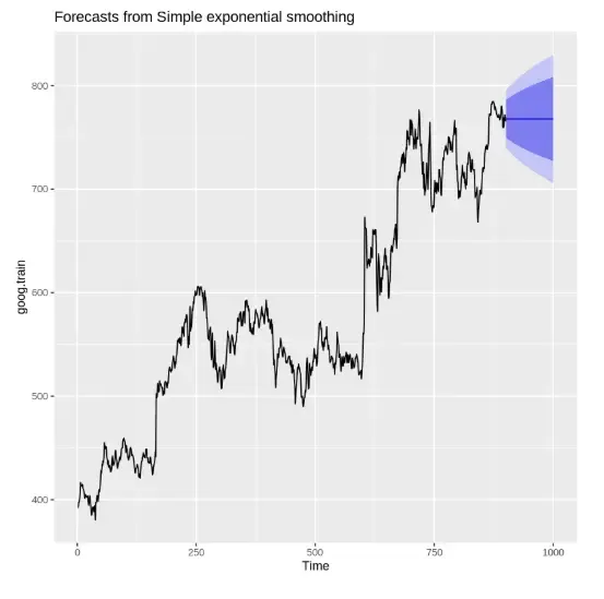
Output
**Step 5: Removing trend and reapplying SES
We use diff() to remove trend and then reapply SES.
- **diff(): differences the series to remove trend.
- **autoplot(): visualizes the time series and forecasts. R `
goog.dif <- diff(goog.train) autoplot(goog.dif) ses.goog.dif <- ses(goog.dif, alpha = 0.2, h = 100) autoplot(ses.goog.dif)
`
**Output:
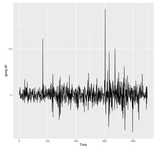
Output
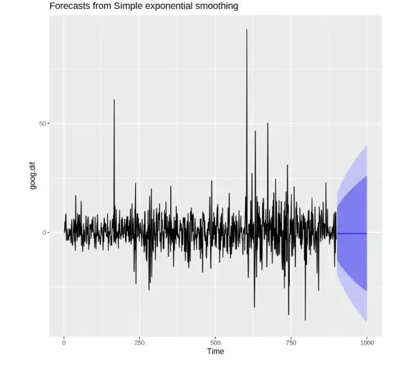
Output
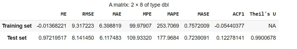
**Step 6: Evaluating the model performance
We difference the test set and evaluate accuracy using accuracy(). It evaluates model performance using metrics like RMSE, MAE.
R `
goog.dif.test <- diff(goog.test) accuracy(ses.goog.dif, goog.dif.test)
`
**Output:
Output
**Step 7: Finding the optimal alpha value
We test multiple alpha values from 0.01 to 0.99 and record RMSE for each.
- **seq(): generates a sequence of numbers.
- **accuracy()[2,2]: extracts test RMSE.
- **ggplot(): plots RMSE vs. alpha values. R `
goog.dif <- diff(goog[1:180]) goog.dif.test <- diff(goog[181:200])
alpha <- seq(0.01, 0.99, by = 0.01) RMSE <- map_dbl(alpha, ~accuracy(ses(goog.dif, alpha = .x, h = length(goog.dif.test)), goog.dif.test)[2, 2])
alpha.fit <- tibble(alpha, RMSE) ggplot(alpha.fit, aes(alpha, RMSE)) + geom_line() + geom_point(data = filter(alpha.fit, RMSE == min(RMSE)), color = "red", size = 2) + labs(title = "Optimal Alpha for SES", x = "Alpha", y = "RMSE")
`
**Output:
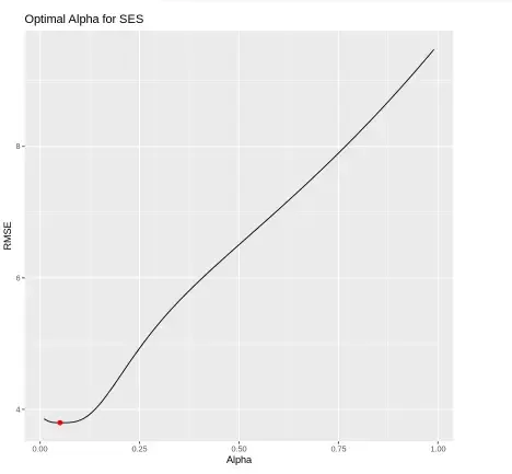
Output
**Step 8: Re-fitting SES with optimal alpha and visualizing predictions
We re-fit the SES model using the optimal alpha = 0.05 and compare the predicted values with the actual test data using a line plot.
- **ses(): refits the model using the best alpha value.
- **accuracy(): checks the model’s performance on the test set.
- **autoplot(): visualizes the original and predicted series.
- **autolayer(): overlays the forecast on the actual data. R `
ses.goog.opt <- ses(goog.dif, alpha = 0.05, h = 100) accuracy(ses.goog.opt, goog.dif.test)
start_time_for_goog_dif_test <- time(goog)[182] goog.dif.test_ts <- ts(goog.dif.test, start = start_time_for_goog_dif_test, frequency = frequency(goog))
p2 <- autoplot(goog.dif.test_ts) + autolayer(ses.goog.opt, alpha = 0.5) + ggtitle("Predicted vs. actuals for the test data set") p2
`
**Output:
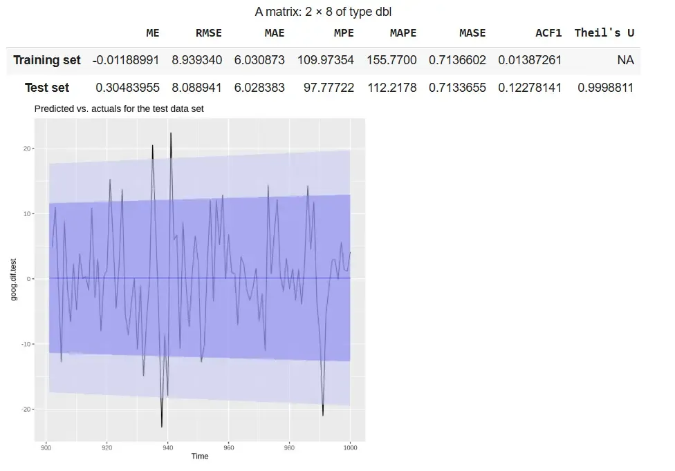
Output
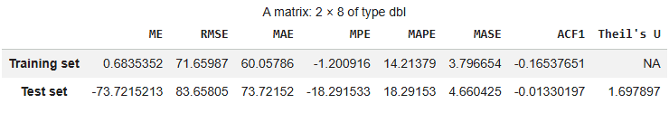
The output shows that the refitted SES model with alpha = 0.05 demonstrates **stable performance, with RMSE and MAE values being similar across training and test sets. The plot indicates that the forecast follows the overall pattern of the actual differenced data within the confidence intervals.
- **RMSE and MAE: Indicate stable model performance
- **Plot: Forecast aligns reasonably well with actual values
- **Theil’s U ≈ 1: Performance is comparable to a naive forecast
2. Holt's Method (Double Exponential Smoothing)
While Simple Exponential Smoothing (SES) works well for data without trend, it cannot account for long-term trends in a time series. Holt's Method, also known as Double Exponential Smoothing, extends SES by incorporating a trend component, making it suitable for datasets that exhibit a trend but no seasonality.
This method uses two smoothing parameters:
- Alpha (\alpha) for smoothing the level of the series.
- Beta (\beta) for smoothing the trend (rate of change).
Holt’s Method allows forecasting both the current level and the trend, providing more accurate predictions for trending time series data. At each time step, the level and trend are updated recursively as:
s_t = \alpha x_t + (1 - \alpha) (s_{t-1} + b_{t-1})
b_t = \beta (s_t - s_{t-1}) + (1 - \beta) b_{t-1}
The forecast for h periods ahead is then:
x_{t+h} = s_t + h \cdot b_t
where
- x_{t+h}: orecast for h periods ahead
- s_{t}: smoothed level at time t
- b_{t}: estimated trend at time t
- \alpha,\beta: smoothing parameters
- h: number of periods ahead
Step By Step Implementation
We will implement Holt’s Method in R to forecast time series data that contains a trend but no seasonality. Unlike Simple Exponential Smoothing (SES), Holt’s Method uses two parameters: alpha for level and beta for trend to adapt to upward or downward movements in the data.
**Step 1: Installing the required packages
We install the required packages to access built-in time series datasets and forecasting functions.
- **install.packages(): used to install external packages from CRAN. R `
install.packages("fpp2") install.packages("tidyverse")
`
**Step 2: Loading the required packages
We will load the necessary libraries.
- **library(): loads a package into the R environment.
- **fpp2: provides datasets and forecasting models including holt().
- **tidyverse: used for data manipulation and plotting. R `
library(tidyverse) library(fpp2)
`
**Step 3: Creating training and testing datasets
We split the goog dataset into training and test sets using window(). It used to extract specific time segments from a time series.
R `
goog.train <- window(goog, end = 900) goog.test <- window(goog, start = 901)
`
**Step 4: Finding the optimal beta value
We loop through beta values from 0.0001 to 0.5 to find the value that minimizes RMSE on the test set.
- **holt(): fits Holt’s method to the data.
- **accuracy(): evaluates the forecast accuracy.
- **ggplot(): plots RMSE values for visual comparison.
- **beta: the smoothing parameter for the trend component. R `
beta <- seq(0.0001, 0.5, by = 0.01) RMSE <- NA
for(i in seq_along(beta)) { fit <- holt(goog.train, beta = beta[i], h = 100) RMSE[i] <- accuracy(fit, goog.test)[2,2] }
beta.fit <- data.frame(beta, RMSE) beta.min <- filter(beta.fit, RMSE == min(RMSE))
library(ggplot2)
ggplot(beta.fit, aes(beta, RMSE)) + geom_line(color = "steelblue") + geom_point(data = beta.min, aes(beta, RMSE), color = "red", size = 3) + labs(title = "RMSE vs Beta (Holt's Method)", x = "Beta", y = "RMSE") + theme_minimal()
`
**Output:

Output
The plot shows RMSE against beta values, highlighting the optimal beta (~0.0601) that minimizes forecasting error in Holt’s method.
**Step 5: Applying Holt’s method and checking accuracy
We apply Holt’s method using the default parameters and measure the model’s performance.
- **holt(): performs forecasting with default optimized alpha and beta.
- **h: number of periods to forecast.
- **accuracy(): prints error metrics for both training and test sets. C++ `
holt.goog <- holt(goog.train, h = 100) accuracy(holt.goog, goog.test)
`
**Output:
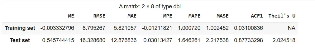
Output
**Step 6: Plotting original vs. optimized Holt’s models side by side
We visualize and compare the forecast from the original Holt’s model and the optimized Holt’s model (with tuned beta).
- **autoplot(): creates plots of the forecast objects.
- **grid.arrange(): displays both plots next to each other. R `
holt.goog <- holt(goog.train, h = 100) holt.goog.opt <- holt(goog.train, beta = 0.0601, h = 100)
install.packages("gridExtra") library(gridExtra)
p1 <- autoplot(holt.goog) + ggtitle("Original Holt's Model") + theme_minimal()
p2 <- autoplot(holt.goog.opt) + ggtitle("Optimal Holt's Model") + theme_minimal()
grid.arrange(p1, p2, ncol = 2)
`
**Output:
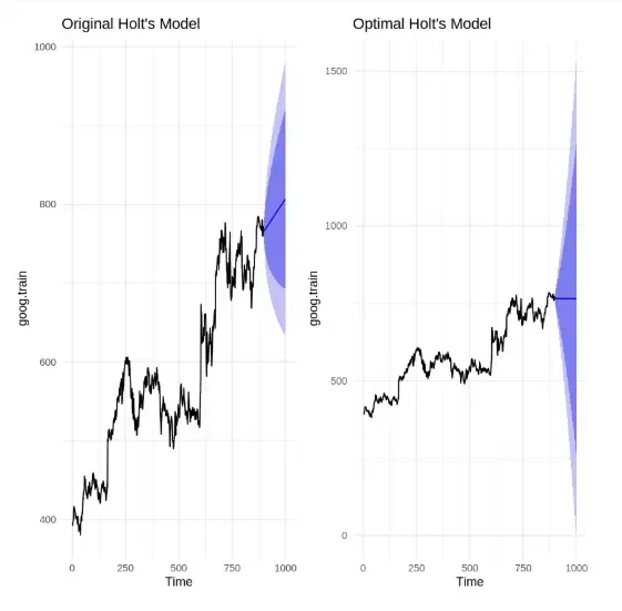
Output
The comparison shows that the original Holt’s model has a sharper trend and narrower confidence interval, while the optimized model (\beta = 0.0601) produces a more conservative forecast with a wider confidence band, reflecting dampened trend and increased uncertainty.
3. Holt-Winters Seasonal Method (Triple Exponential Smoothing)
The Holt-Winters Seasonal Method is used for time series data that exhibits both trend and seasonality. It extends Holt’s method by including a seasonal component, allowing more accurate forecasting for complex datasets. The method can be applied as Additive for constant seasonal variations or Multiplicative when seasonal effects change proportionally with the series level.
Holt-Winters smoothing uses three parameters:
- \alpha (alpha): for the level of the series
- \beta (beta): for the trend
- \gamma (gamma): for the seasonal component
The method updates these components recursively using the following formulas:
**1. Initial level
s_0 = x_0
**2. Level update
s_t = \alpha \frac{x_t}{c_{t-L}} + (1 - \alpha) (s_{t-1} + b_{t-1})
**3. Trend update
b_t = \beta (s_t - s_{t-1}) + (1 - \beta) b_{t-1}
**4. Seasonal component update
c_t = \gamma \frac{x_t}{s_t} + (1 - \gamma) c_{t-L}
where
- s_{t}: smoothed level at time t
- b_{t}: estimated trend at time t
- c_{t}: seasonal component at time t
- x_{t}: actual observation at time t
- L: length of the seasonal cycle
- \alpha, \beta, \gamma: smoothing parameters (0 < value < 1)
Step By Step Implementation
Here we implement Holt Winter’s Seasonal Method to forecast time series data that shows both trend and seasonality. The method uses three smoothing parameters: alpha for level, beta for trend and gamma for seasonality and supports both Additive and Multiplicative models depending on the pattern in the data.
**Step 1: Installing the required packages
We install the necessary packages for time series analysis and visualization.
- **install.packages(): used to install CRAN packages.
- **fpp2: includes the ets() and datasets like qcement.
- **tidyverse: used for plotting and data manipulation. R `
install.packages("fpp2") install.packages("tidyverse")
`
**Step 2: Loading the required packages
Load the installed packages into the current session. library() loads the specified package.
R `
library(fpp2) library(tidyverse)
`
**Step 3: Creating training and testing datasets
Split the qcement dataset into training and test sets to evaluate model performance. window() extracts specific segments from a time series object.
R `
qcement.train <- window(qcement, end = c(2012, 4)) qcement.test <- window(qcement, start = c(2013, 1))
`
**Step 4: Applying the additive Holt-Winters model
We apply the additive seasonal model using ets() with model set to "AAA".
- **ets(): fits exponential smoothing models to time series data.
- **model = "AAA": specifies Additive Error, Additive Trend, Additive Seasonality.
- **summary(): displays fitted model details and smoothing parameters.
- **checkresiduals(): performs residual analysis.
- **forecast(): generates future forecasts.
- **accuracy(): evaluates model predictions. R `
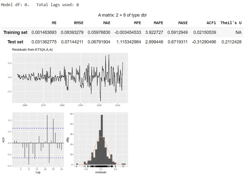
qcement.hw <- ets(qcement.train, model = "AAA") summary(qcement.hw) checkresiduals(qcement.hw)
qcement.f1 <- forecast(qcement.hw, h = 8) accuracy(qcement.f1, qcement.test)
`
**Output:
Output
The additive model delivers accurate forecasts with stable seasonality and low errors, despite slight residual autocorrelation.
**Step 5: Applying the multiplicative Holt-Winters model
We apply the multiplicative model using ets() with model set to "MAM".
- **model = "MAM": specifies Multiplicative Error, Additive Trend, Multiplicative Seasonality.
- **checkresiduals(): checks residual patterns and model fit.
- **forecast(): projects future values.
- **accuracy(): checks predictive accuracy. R `
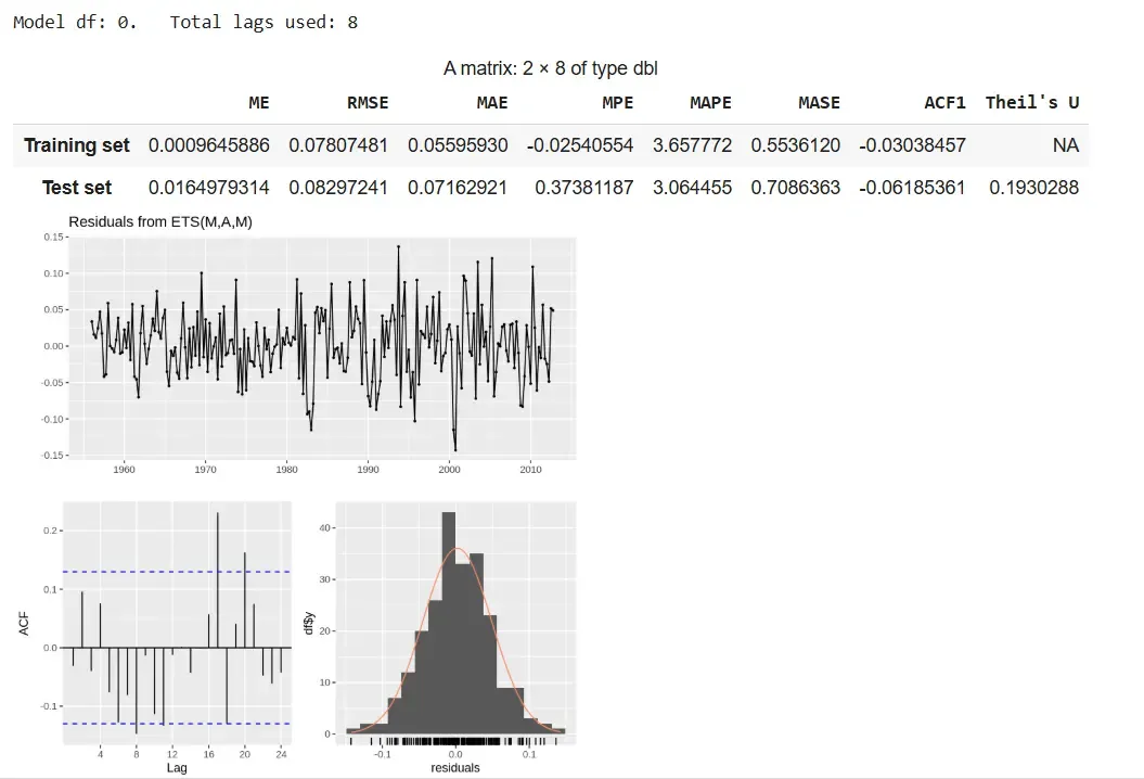
qcement.hw2 <- ets(qcement.train, model = "MAM") checkresiduals(qcement.hw2)
qcement.f6 <- forecast(qcement.hw2, h = 8) accuracy(qcement.f6, qcement.test)
`
**Output:
Output
The multiplicative model provides better accuracy with scaling seasonality but shows slight residual autocorrelation.
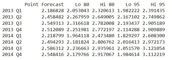
**Step 6: Viewing forecasted values
We view the forecast output including the point predictions and confidence intervals for future quarters. qcement.f6 shows predictions for each future period along with 80% and 95% prediction intervals.
R `
qcement.f6
`
**Output:
Output
The output displays predicted values for 2013 Q1 to 2014 Q4 using the additive model. The values follow a consistent seasonal trend and highlight the growing uncertainty across periods.
- Forecast values show seasonally adjusted trends.
- Interval width increases gradually, indicating uncertainty over time.
- Predictions align well with the training pattern due to additive structure.
4. Damped Trend Method
The Damped Trend Method is an extension of Holt’s Exponential Smoothing that is used for time series with a trend, but where the trend is expected to slow down or level off over time. Unlike Holt’s method, which projects the trend indefinitely, the damped trend introduces a damping factor (\phi) that reduces the influence of the trend in future forecasts, making long-term predictions more realistic.
This method uses three components:
- Level (\alpha): smooths the current value of the series
- Trend (\beta): smooths the estimated trend
- Damping factor (\phi): reduces the trend effect over time (0 < \phi < 1)
**Step By Step Implementation
**Step 1: Install and load required packages
Install and load required packages to work with time series data and forecasting functions.
R `
install.packages("fpp2") install.packages("forecast") library(fpp2) library(forecast)
`
**Step 2: Prepare the dataset
Here we use ausbeer dataset as an example, which has a clear trend. We split it into training and test sets for evaluation.
R `
beer.train <- window(ausbeer, end = c(2007, 4))
beer.test <- window(ausbeer, start = c(2008, 1))
`
**Step 3: Fit the Damped Trend Model
Fit Holt’s method with a damping factor so the trend gradually slows over time.
R `
damped.model <- holt(beer.train, damped = TRUE, alpha = 0.8, beta = 0.2, phi = 0.9, h = length(beer.test))
`
**Step 4: Visualize the forecast
Plot the training data, actual test data and the model forecast to see how well the damped trend predicts future values.
R `
autoplot(beer.train, series = "Training Data") + autolayer(beer.test, series = "Actual Test Data") + autolayer(damped.model$mean, series = "Damped Trend Forecast") + ggtitle("Damped Trend Forecast vs Actuals") + xlab("Year") + ylab("Beer Production") + guides(colour = guide_legend(title = "Series"))
`
**Output:
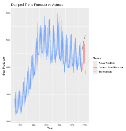
Output
**Step 5: Evaluate forecast accuracy
We calculate accuracy metrics like RMSE, MAE and MAPE to check how close the forecast is to the actual test data.
R `
accuracy(damped.model, beer.test)
`
**Output:
Output
Download full code from here
**Applications
Adding a real-world applications section helps readers understand where and why exponential smoothing is used practically:
- **Financial Forecasting: Predicting stock prices, interest rates and exchange rates.
- **Sales and Demand Forecasting: Estimating product demand in retail, e-commerce and supply chain.
- **Inventory Management: Anticipating inventory needs to reduce overstock or stockouts.
- **Weather Prediction: Forecasting temperature or rainfall based on historical data.
- **Energy Load Forecasting: Estimating future electricity or gas demand for efficient energy management.
Advantages
- **Simple and Fast: Easy to implement with minimal computational cost.
- **Responsive to Recent Data: Gives more weight to recent observations for better short-term forecasting.
- **Flexible: Variants like Holt’s and Holt-Winters handle trend and seasonality.
Limitation
- Not suitable for complex patterns like irregular seasonality or sudden structural changes.
- Forecast accuracy declines over longer horizons due to increasing uncertainty.
- Poor choice of \alpha,\beta, or \gamma can lead to inaccurate forecasts.