Feature Engineering in R Programming (original) (raw)
Last Updated : 13 Dec, 2025
Feature Engineering in R means creating new features or modifying existing ones to make models work better. It includes cleaning, transforming, scaling, encoding and selecting features for machine learning.
- Helps models understand data better
- Removes noise and unwanted patterns
- Converts raw data into useful inputs
- Works with both numeric and categorical features
In R, this is done using packages like dplyr, tidyr, caret and data.table.
Sample Dataset
R `
df <- data.frame( age = c(23, 45, 35, 62, 18), income = c(30000, 60000, 45000, 80000, 20000), gender = c("Male", "Female", "Female", "Male", "Male"), city = c("A", "B", "A", "C", "B") ) df
`
**Output:
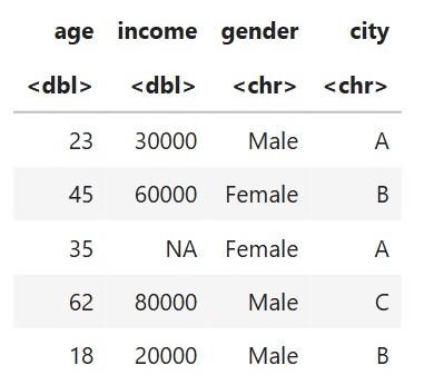
Sample Dataset
This dataset has:
- **Numeric features: age, income
- **Categorical features: gender, city
We will use this small data to explain each concept.
1. Handling Missing Values
The dataset contains a missing value in income.
**Example (add NA for explanation):
R `
df$income[is.na(df$income)] <- mean(df$income, na.rm = TRUE) df
`
**Output:
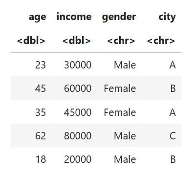
Dataset After Handling Missing Values
**Explanation:
mean(..., na.rm = TRUE)calculates mean without NA.- Replaces missing entry with the average income.
2. Encoding Categorical Variables
**Label Encoding (for binary categories: gender)
R `
df$gender_num <- ifelse(df$gender == "Male", 1, 0) df
`
**Output:
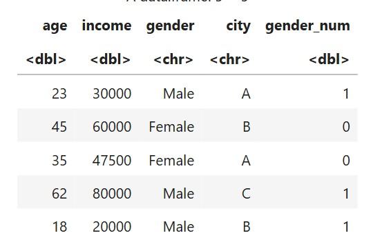
Dataset After Label Encoding
**Explanation:
- Male = 1
- Female = 0
**One-Hot Encoding (for multi-class: city)
R `
ohe <- model.matrix(~ city - 1, data = df) df <- cbind(df, ohe) df
`
**Output:
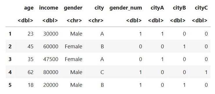
Dataset After One hot encoding
**Explanation:
City A, B and C become separate columns:
- cityA
- cityB
- cityC
Each gets 0/1 depending on membership.
3. Feature Scaling
Scaling helps numeric values stay on similar ranges.
**Using standard scaling (mean = 0, sd = 1)
R `
df$age_scaled <- scale(df$age) df$income_scaled <- scale(df$income) df
`
**Output:
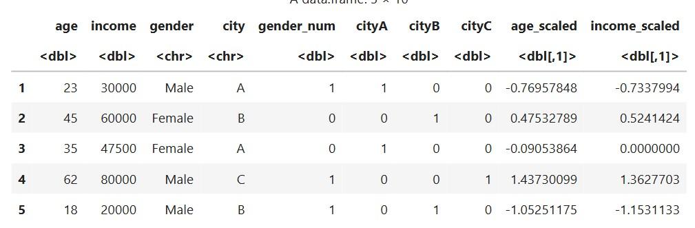
Dataset after Using standard scaling
**Explanation:
- Makes numeric features easier for algorithms like KNN, SVM, etc.
4. Binning (Feature Transformation)
Create age groups:
R `
df$age_group <- cut( df$age, breaks = c(0, 25, 50, 100), labels = c("Young", "Middle", "Senior") ) df
`
**Output:
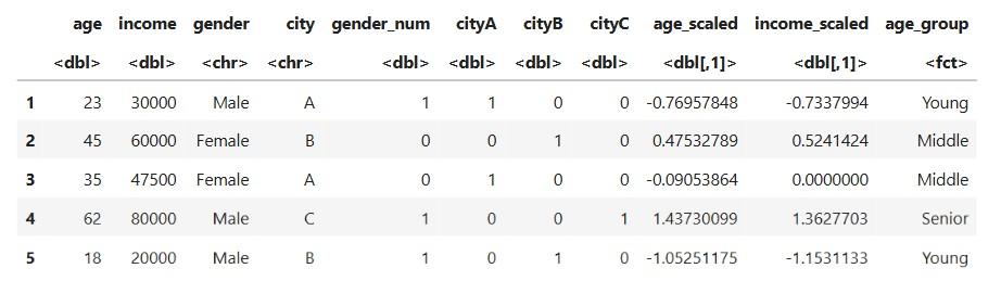
Dataset after Feature Transformation
**Explanation:
- Converts continuous age into categories
- Helps models see pattern in ranges
5. Feature Construction
**Create a new feature: income per year of age
R `
df$income_per_age <- df$income / df$age df
`
**Output:
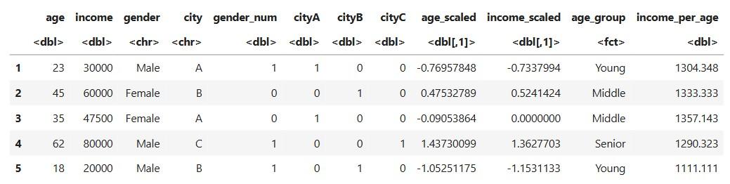
Dataset after Feature Construction
6. Removing Skewness
Apply log transformation to reduce skew in income:
R `
df$income_log <- log(df$income + 1) df
`
**Output:
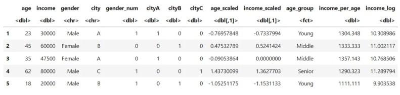
Dataset after Removing Skewness
**Explanation:
- Helps stabilize values
- Makes distribution smoother
7. Final Cleaned Feature-Enhanced Dataset
After all steps, the dataset now looks like this:
- original variables (age, income, gender, city)
- encoded variables (gender_num, cityA, cityB, cityC)
- scaled variables (age_scaled, income_scaled)
- transformed variables (income_log, age_group)
- constructed feature (income_per_age)
This feature rich dataset is now ready for modeling.