Fisher’s FTest in R Programming (original) (raw)

Last Updated : 15 Jul, 2025

In this article, we will delve into the fundamental concepts of the F-Test, its applications, assumptions, and how to perform it using R programming. We will also provide a step-by-step guide with examples and visualizations to help you master the F-Test in the R Programming Language.

What is Fisher’s F-Test?

Fisher's F-test is a statistical method used to compare the variances of two independent samples to determine if they come from populations with the same variance. It tests the ratio of two sample variances to see if they differ significantly. The F-test is the foundation for other advanced statistical tests, such as ANOVA (Analysis of Variance).

F = Larger Sample Variance / Smaller Sample Variance

**When to Use the F-Test?

• To compare the variability between two groups.
• To test for homogeneity of variances, which is an essential assumption in various statistical methods, like ANOVA or t-tests.

**Assumptions of the F-Test

Before performing the F-Test, certain assumptions must be met:

1. **Normality: Both samples should be normally distributed.
2. **Independence: The two samples should be independent of each other.
3. **Ratio Scale: Data should be measured on an interval or ratio scale.

Now we will discuss How to perform Fisher’s F-Test in R Programming Langauge.

**Approach 1: Using the var.test() Function

R provides a built-in function var.test() that performs the F-Test easily.

var.test(x, y, alternative = "two.sided")

**Where,

• **x, y: numeric vectors
• **alternative: a character string specifying the alternative hypothesis.

Suppose we have two samples of data representing the weights of two different groups of individuals:

r `

Sample data

group1 <- c(15.2, 16.5, 14.8, 16.9, 15.5, 15.8) group2 <- c(14.0, 13.8, 15.2, 13.9, 14.1, 14.5)

Perform the F-Test

f_test_result <- var.test(group1, group2)

Display the result

print(f_test_result)

`

**Output:

F test to compare two variances

data: group1 and group2
F = 2.2897, num df = 5, denom df = 5, p-value = 0.3844
alternative hypothesis: true ratio of variances is not equal to 1
95 percent confidence interval:
0.3203995 16.3630488
sample estimates:
ratio of variances
2.289697

The var.test() function output provides:

• The F statistic value
• Degrees of freedom (df)
• p-value

If the p-value is less than the chosen significance level (commonly 0.05), we reject the null hypothesis, indicating a significant difference in variances.

**Approach 2: Manual Calculation of F-Test in R

You can calculate the F-Test manually using R to understand the process more deeply.

r `

Calculate variances

var_group1 <- var(group1) var_group2 <- var(group2)

Calculate F statistic

f_value <- var_group1 / var_group2

Display F statistic

cat("F Statistic:", f_value, "\n")

`

**Output:

F Statistic: 2.289697

• **F-value: Indicates the ratio of variances. Higher F-values suggest more considerable differences.
• **p-value: The probability of observing the F statistic under the null hypothesis. If the p-value is low (< 0.05), reject H₀.

**Visualizing the F-Test Distribution

You can visualize the F distribution using R's plotting functions to better understand the test's results.

R `

Visualize F-distribution

curve(df(x, df1 = 5, df2 = 5), from = 0, to = 5, col = "blue", lwd = 2, xlab = "F-value", ylab = "Density", main = "F-Distribution with df1=5, df2=5")

`

**Output:

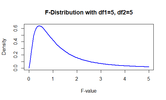
Fisher’s F-Test in R Programming

**Conclusion

Fisher’s F-Test is a powerful statistical method for comparing variances between two groups. It is easy to implement in R using the var.test() function or manually calculating it. However, it's essential to meet the assumptions and be cautious of its limitations to ensure accurate results.