Fuzzy Clustering in R (original) (raw)
Last Updated : 28 Jun, 2025
Clustering is an unsupervised machine learning technique that is used to identify similarities and patterns within data points by grouping similar points based on their features. These points can belong to different clusters simultaneously. Fuzzy clustering is a clustering technique where each data point can belong to multiple clusters with varying degrees of membership. In normal clustering, each data point goes into only one group, while in fuzzy clustering, a point can be shared between groups to different degrees.
Understanding Fuzzy Clustering
In real-world scenarios, data points may naturally belong to more than one cluster. Fuzzy clustering addresses this by allowing data points to belong to multiple clusters at the same time. Its key advantages over normal clustering include:
- **Soft Boundaries: Fuzzy clustering allows data points to belong to multiple clusters simultaneously, offering a more realistic approach to data classification.
- **Robustness to Noisy Data: It handles noisy and ambiguous data better than normal clustering methods.
- **Flexibility: It provides the flexibility for data points to be part of more than one cluster, making it suitable for analyzing complex data structures.
Difference between Normal and Fuzzy Clustering
| **Factor | **Normal Clustering | **Fuzzy Clustering |
|---|---|---|
| Partitioning | Hard Partitioning, data points can belong to only one cluster. | Soft Partitioning, data points can belong to multiple clusters. |
| Membership | Data points can either belong to one cluster or none at all. | Data points can belong to multiple clusters simultaneously. |
| Representation | represented by centroids. | represented by centroids with degrees of membership. |
| Suitable dataset | Dataset with distinct boundaries. | Dataset with overlapping observations. |
| Algorithm used | K-means, Hierarchical clustering. | Fuzzy C -means, Gustafson-Kessel algorithm. |
| Implementation | Easier to implement since the dataset is not complex. | Difficult to Implement since dataset has overlapping observations. |
Fuzzy Clustering in R using Customer Segmentation Dataset
In this example we will apply fuzzy clustering on a Sample sales dataset.
You can download the dataset from here.
1. Loading Required Libraries
We are installing and loading the libraries that provide necessary functions for clustering and visualization.
- **e1071: Contains the cmeans() function used for fuzzy c-means clustering.
- **cluster: Provides clustering algorithms like pam() and evaluation tools.
- **factoextra: Helps in visualizing clustering results in a clear and effective way. R `
install.packages("e1071") install.packages("cluster") install.packages("factoextra")
library(e1071) library(cluster) library(factoextra)
`
2. Loading the Dataset
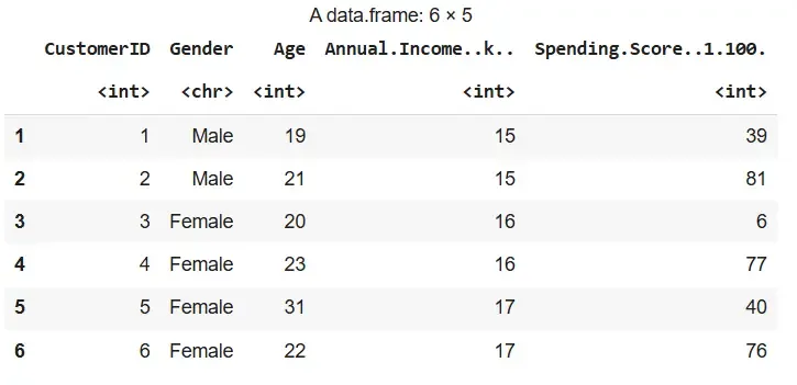
We are reading the CSV file containing the data and inspecting the first few rows.
- **read.csv(): Loads the dataset from the given file path.
- **head(): Displays the first few rows of the data to get an overview. R `
data <- read.csv("/content/Mall_Customers.csv")
head(data)
`
**Output:
Output
3. Data Preprocessing
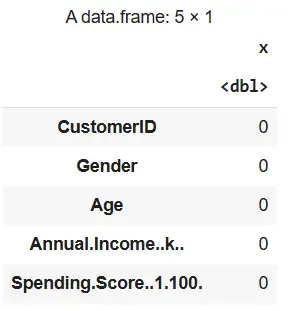
We are cleaning the dataset to ensure accuracy in clustering.
- **is.na(): Identifies NA values in the dataset.
- **colSums(is.na(data)): Gives the number of missing values per column.
- **na.omit(): Removes rows with missing values. R `
x <- colSums(is.na(data)) x <- as.data.frame(x) x
data<- na.omit(data)
`
**Output:
Output
4. Selecting Data for Clustering
We are choosing relevant features that influence clustering: Age, Income and Spending Score.
R `
data_for_clustering <- data[, c("Age", "Annual.Income..k..", "Spending.Score..1.100.")]
`
5. Applying Fuzzy C-means Clustering
We are performing fuzzy clustering using the cmeans() function from e1071.
- **set.seed(123): Ensures reproducibility.
- **n_cluster: Number of desired clusters.
- **m: Fuzziness coefficient (commonly between 1.5 and 3).
- **result$membership: Stores membership degrees.
- **result$centers: Gives cluster centers. R `
set.seed(123) n_cluster <- 5 m <- 2 result <- cmeans(data_for_clustering, centers = n_cluster, m = m)
fuzzy_membership_matrix <- result$membership
initial_centers <- result$centers final_centers <- t(result$centers)
`
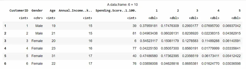
6. Interpreting the Clustering Results
We are combining the fuzzy membership matrix with the original dataset for analysis.
- **cbind(): Merges cluster probabilities with data. R `
cluster_membership <- as.data.frame(result$membership) data_with_clusters <- cbind(data, cluster_membership) head(data_with_clusters)
`
**Output:
Output
7. Evaluating the Clustering Quality
The quality of a cluster refers to how well-separated and distinct the clusters are from each other and how cohesive the data points within each cluster are. A high-quality cluster should have tightly grouped points and be well-separated from other clusters. We will evaluate the quality of the formed clusters using the following approach:
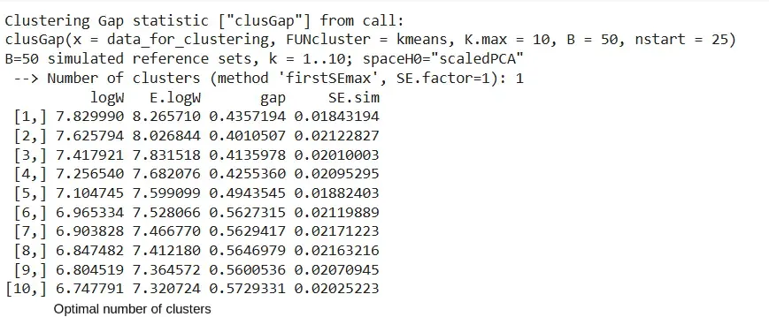
7.1. Using Gap Statistic
We are computing the gap statistic to determine the optimal number of clusters by comparing the model’s performance with random uniform distribution.
- **clusGap(): Computes the gap statistic for different values of k.
- **FUN = kmeans: Uses k-means clustering for computation.
- **nstart = 25: Runs k-means 25 times for each value of k.
- **K.max = 10: Evaluates up to 10 clusters.
- **B = 50: Number of Monte Carlo simulations.
- **print(): Displays the gap statistic values.
- **fviz_gap_stat(): Visualizes the gap statistic results with error bars. R `
library(cluster)
gap_stat <- clusGap(data_for_clustering, FUN = kmeans, nstart = 25, K.max = 10, B = 50)
print(gap_stat)
fviz_gap_stat(gap_stat)
`
**Output:
Output
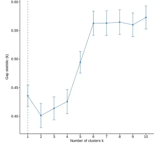
Output
7.2. Using Davies-Bouldin Index
We are calculating the Davies-Bouldin Index to measure intra-cluster similarity and inter-cluster separation.
- **index.DB(): Calculates the Davies-Bouldin index.
- **data_for_clustering: The input data.
- **km_res$cluster: Cluster labels from k-means.
- **centrotypes = "centroids": Uses centroid-based distance.
- **print(): Displays the DB index value. R `
install.packages("clusterSim") library(clusterSim)
set.seed(123) km_res <- kmeans(data_for_clustering, centers = 5, nstart = 25)
db_index <- index.DB(data_for_clustering, km_res$cluster, centrotypes = "centroids")
print(db_index$DB)
`
**Output:
[1] 0.884653
7.3. Using Calinski-Harabasz Index
We are computing the Calinski-Harabasz (CH) Index to evaluate the ratio of between-cluster dispersion to within-cluster dispersion.
- **index.G1(): Computes the CH index.
- **data_for_clustering: Input dataset.
- **km_res$cluster: Cluster labels from k-means.
- **print(): Displays the CH index value. R `
ch_index <- index.G1(data_for_clustering, km_res$cluster)
print(ch_index)
`
**Output:
[1] 151.0439
8. Visualizing the Clustering Results
We will visualize the clustering results to better understand the distribution and separation of the formed clusters.
8.1. 2D Scatter Plot
We are plotting customer data colored by their fuzzy cluster assignment for easy interpretation.
- **apply(..., which.max): Assigns each data point to the cluster where it has the highest membership score.
- **ggplot(): Initializes a ggplot object.
- **aes(): Defines aesthetics like x, y and color.
- **geom_point(): Plots scatter points.
- **labs(): Adds axis labels and title. R `
data_with_clusters$Cluster <- apply(result$membership, 1, which.max)
ggplot(data_with_clusters, aes(x = Annual.Income..k.., y = Spending.Score..1.100., color = as.factor(Cluster))) + geom_point(size = 2) + labs(title = "Fuzzy C-means Clustering", x = "Annual Income (k$)", y = "Spending Score")
`
**Output:
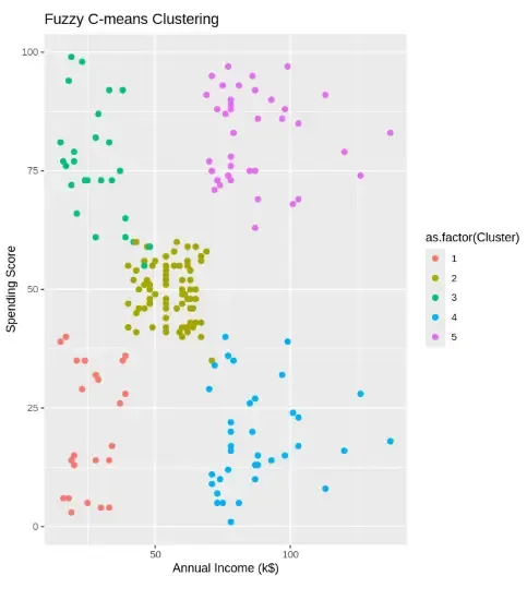
Output
7.2. Pairwise Variable Relationship Plot
We are creating pairwise scatter plots to study the relationship between clustering variables.
- **pairs(): Plots a matrix of scatterplots for each variable combination.
- **pch = 16: Defines point shape.
- **col = as.numeric(...): Colors points based on cluster membership. R `
pairs(data_for_clustering, pch = 16, col = as.numeric(result$cluster))
`
**Output:
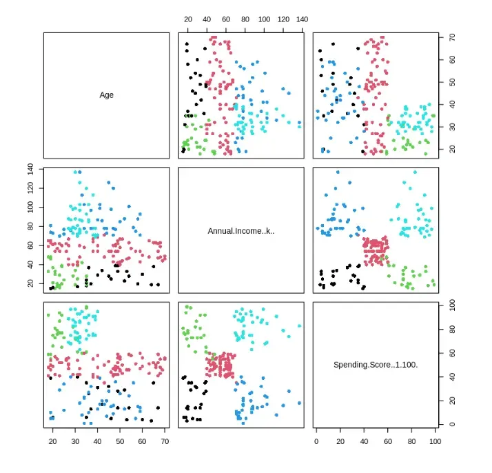
Output
7.3. Clusplot for 2D Cluster Projection
We are visualizing clusters in 2D space using dimensionality reduction.
- **clusplot(): generates a cluster plot using principal component analysis (PCA).
- **color = TRUE: Colors clusters differently.
- **shade = TRUE: Adds shaded areas around clusters.
- **labels = 2: Displays labels for clusters.
- **lines = 0: Removes connecting lines. R `
clusplot(data_for_clustering, result$cluster, color = TRUE, shade = TRUE, labels = 2, lines = 0)
`
**Output:

Output
This plot shows how the data points are grouped into clear clusters in 2D, capturing about 77.57% of the original data’s information.