Gamma Distribution in R Programming dgamma(), pgamma(), qgamma(), and rgamma() Functions (original) (raw)

Last Updated : 15 Jul, 2025

The Gamma distribution in R Programming Language is defined as a two-parameter family of continuous probability distributions which is used in exponential distribution, Erlang distribution and chi-squared distribution.

Mathematical Implementation of the Gamma Distribution

A random variable X is said to follow a Gamma distribution with shape parameter \alpha (alpha) and rate parameter\beta (beta) if its probability density function (PDF) is defined as:

f(x; \alpha, \beta) = \frac{\beta^\alpha}{\Gamma(\alpha)} x^{\alpha - 1} e^{-\beta x}, \quad \text{for } x > 0, \alpha, \beta > 0

where:

• \alpha > 0is the **shape parameter.
• \beta > 0 is the **rate parameter (sometimes the scale parameter\theta = 1/\beta is used).
• \Gamma(\alpha) is the gamma function, defined as\Gamma(\alpha) = \int_0^\infty t^{\alpha - 1} e^{-t} dt

**Key properties:

• ****Mean:**\mu = \frac{\alpha}{\beta}
• ****Variance:**\sigma^2 = \frac{\alpha}{\beta^2}

Implementation of Gamma Distribution Functions in R

We will implement various gamma distribution functions available in the R programming language and understand their interpretation through visualizations.

1. dgamma() Function

The **dgamma() function in R calculates the **probability density function (PDF) of the Gamma distribution at specified values.

**Syntax:

dgamma(x_dgamma, shape)

**Parameters:

• x_dgamma: A numeric vector of values at which to evaluate the gamma density.
• shape: The shape parameter (α\alphaα) of the Gamma distribution (must be positive).

**Example :

We generate a sequence of values from 0 to 2 and compute the gamma probability density function (PDF) with a shape parameter of 6 at those points. Finally, we plot the computed gamma density values to visualize the distribution.

R `

x_dgamma <- seq(0, 2, by = 0.04)

y_dgamma <- dgamma(x_dgamma, shape = 6)

plot(y_dgamma)

`

**Output :

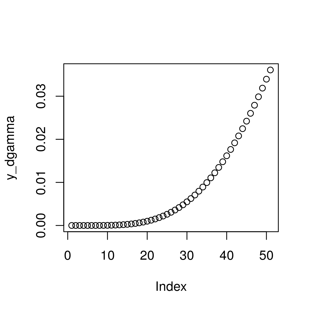
Gamma Distribution in R

2. pgamma() Function

The**pgamma()** function computes the **cumulative distribution function (CDF) of the Gamma distribution at specified values. It returns the probability that a Gamma distributed random variable is less than or equal to each value in the input.

**Syntax:

pgamma(x_pgamma, shape)

**Parameters:

• **x_pgamma: defines gamma function
• **shape: gamma density of input values

Example:

We create a sequence of values from 0 to 2 and calculate the gamma cumulative distribution function (CDF) with shape parameter 6 for those values. Then, we plot the CDF values to visualize the accumulation of probability.

R `

x_pgamma <- seq(0, 2, by = 0.04)

y_pgamma <- pgamma(x_pgamma, shape = 6)

plot(y_pgamma)

`

**Output:

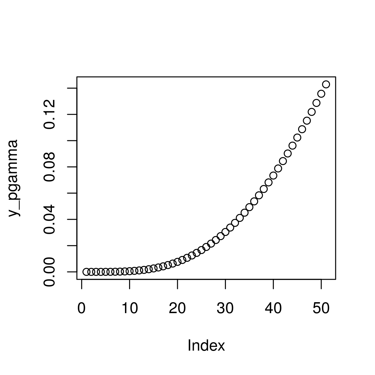
Cumulative Gamma Distribution Function

3. qgamma() Function

The qgamma() function computes the **quantile function (inverse cumulative distribution function) of the Gamma distribution. It returns the value x such that the cumulative probability of the Gamma distribution up to x equals a given probability.

**Syntax:

qgamma(x_qgamma, shape)

**Parameters:

• **x_qgamma: defines gamma function
• **shape: gamma density of input values

**Example:

We generate a sequence of probabilities from 0 to 1 and compute the gamma quantile function (inverse CDF) with a shape parameter of 6 at those probabilities. The resulting quantiles are then plotted to visualize the relationship between cumulative probabilities and their corresponding gamma distribution values.

R `

x_qgamma <- seq(0, 1, by = 0.03)

y_qgamma <- qgamma(x_qgamma, shape = 6)

plot(y_qgamma)

`

**Output:

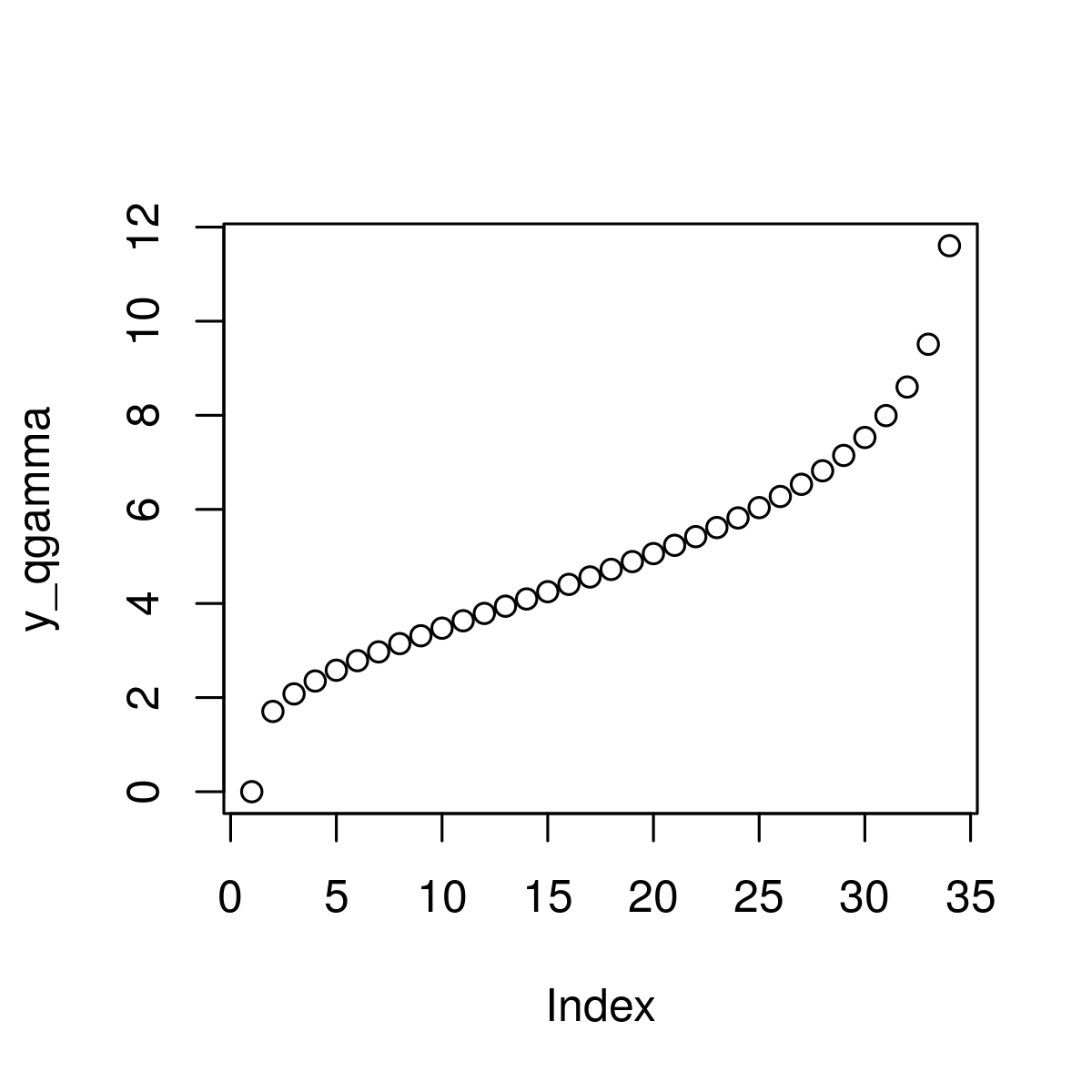
Quantile Function of Gamma Distribution

4. rgamma() Function

The **rgamma()**function generates random numbers drawn from a Gamma distribution. It is commonly used for simulations and modeling when random samples from a Gamma distribution are required.

**Syntax:

rgamma(N, shape)

**Parameters:

• **N: gamma distributed values
• **shape: gamma density of input values

**Example:

We set a seed for reproducibility and generate 800 random values from a gamma distribution with shape parameter 5. A histogram with 500 bins is plotted to visualize the distribution of these random gamma values.

R `

set.seed(1200)

N <- 800

y_rgamma <- rgamma(N, shape = 5)

hist(y_rgamma, breaks = 500, main = "")

`

**Output:

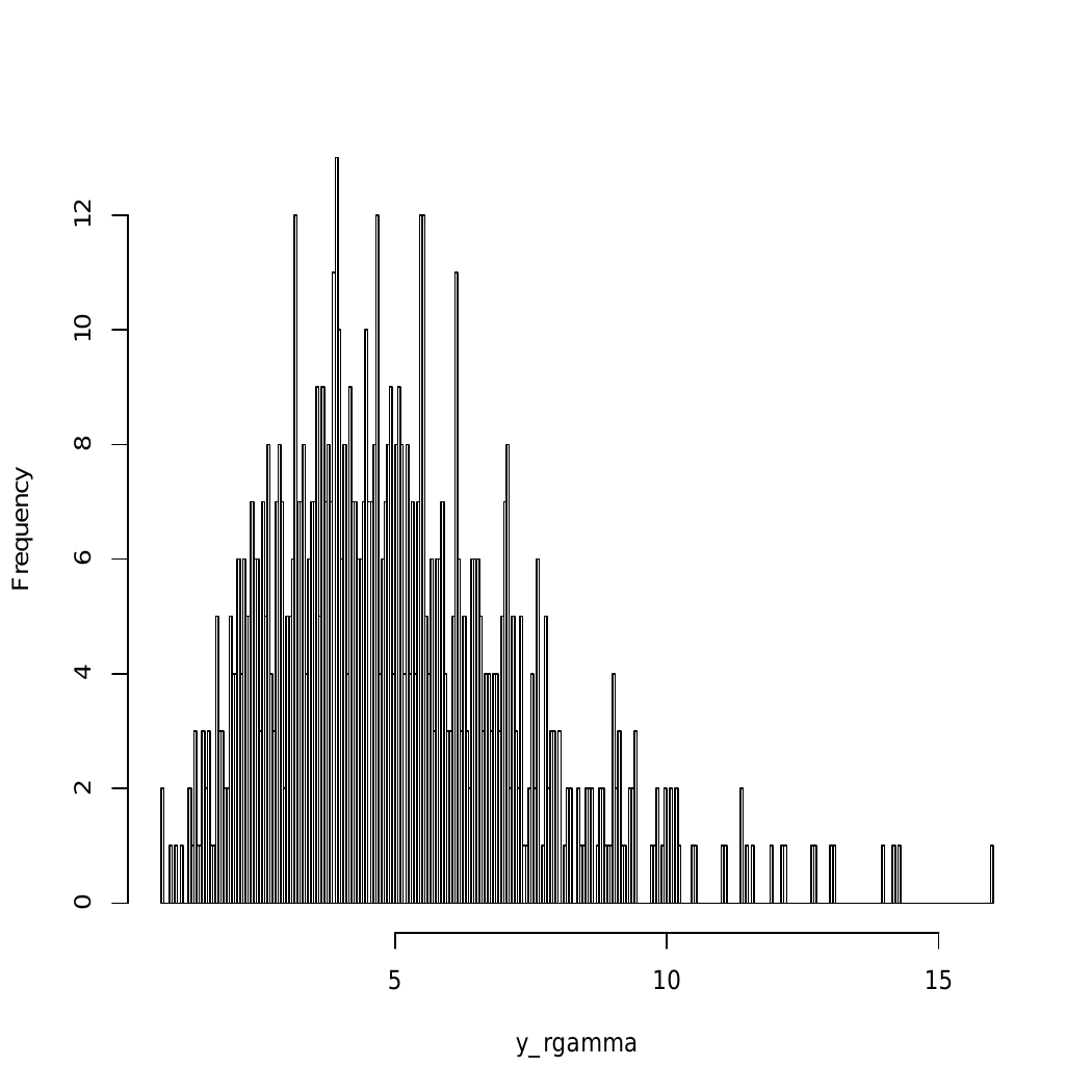
Histogram of 100 Gamma Distributed Numbers

In this article, we explored the key functions of the Gamma distribution in R such as dgamma(), pgamma(), qgamma() and rgamma(). We demonstrated how to use these functions for density calculation, cumulative probabilities, quantile estimation and random number generation.