Generalized Linear Models Using R (original) (raw)
Last Updated : 2 May, 2025
GLMs (Generalized linear models) are a type of statistical model that is extensively used in the analysis of non-normal data, such as count data or binary data. They enable us to describe the connection between one or more predictor variables and a response variable in a flexible manner.
Major components of GLMs
- A probability distribution for the response variable
- A linear predictor function of the predictor variables
- A link function that connects the linear predictor to the response variable's mean.
The probability distribution and link function used is determined by the type of response variable and the research topic at hand. R includes methods for fitting GLMs, such as the glm() function. The user can specify the formula for the model, which contains the response variable and one or more predictor variables, as well as the probability distribution and link function to be used, using this function.
Mathematical Formulation of GLM
In Generalized Linear Models (GLMs), the response variable Yis assumed to follow a distribution from the exponential family. The model relates the expected value of Y, denoted \mu , to the predictors X via a link function:
g(\mu) = X\beta
Here, \beta is the vector of model coefficients and g(\cdot) is a specified link function. The variance of Y is given by:
\text{Var}(Y) = \phi V(\mu)
where V(\mu) is the variance function and \phi is a dispersion parameter.
Classical Linear Regression as a Special Case
In linear regression, Y = X\beta + \epsilon , with \epsilon \sim N(0, \sigma^2), is a special case where:
- g(\mu) = \mu (identity link)
- V(\mu) = 1
- \phi = \sigma^2
Estimation
Model parameters \beta are estimated via maximum likelihood. For observations (x_i, y_i), the likelihood is:
L(\beta) = \prod_{i=1}^n f(y_i \mid \mu_i)
where f(\cdot) is the density function of the assumed distribution and \mu_i is the expected value of Y_i given x_i.
GLM model families
There are several GLM model families depending on the make-up of the response variable. These includes three well-known GLM model families:
- **Binomial: The binomial family is used for binary response variables (i.e., two categories) and assumes a binomial distribution. R `
model <- glm(binary_response_variable ~ predictor_variable1 + predictor_variable2, family = binomial(link = "logit"), data = data)
`
- **Gaussian: This family is used for continuous response variables and assumes a normal distribution. The link function for this family is typically the identity function. R `
model <- glm(response_variable ~ predictor_variable1 + predictor_variable2, family = gaussian(link = "identity"), data = data)
`
- **Gamma: The gamma family is used for continuous response variables that are strictly positive and have a skewed distribution. R `
model <- glm(positive_response_variable ~ predictor_variable1 + predictor_variable2, family = gamma(link = "inverse"), data = data)
`
- **Quasibinomial: When a response variable is binary but has a higher variance than would be predicted by a binomial distribution, the quasibinomial model is utilized. This could happen if the response variable has excessive dispersion or additional variation that the model is not taking into account. R `
model <- glm(response_variable ~ predictor_variable1 + predictor_variable2, family = quasibinomial(), data = data)
`
Building a Generalized Linear Model
1. Loading the Dataset
We will use the "mtcars" dataset in R to illustrate the use of generalized linear models. This dataset includes data on different car models, including mpg, horsepower (hp) and weight. (wt). The response variable will be "mpg," and the predictor factors will be "hp" and "wt."
R `
data(mtcars) head(mtcars)
`
**Output:
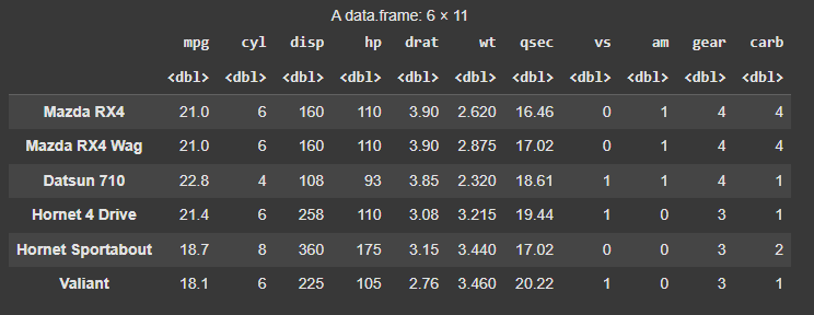
Sample Data
To create a generalized linear model in R, we must first select a suitable probability distribution for the answer variable.
- If the answer variable is binary (e.g., 0 or 1), we could use the Bernoulli distribution.
- If the response variable is a count (for example, the number of vehicles sold), the Poisson distribution may be used.
2. Building the model
To create a generalized linear model in R, use the glm() tool. We must describe the model formula (the response variable and the predictor variables) as well as the probability distribution family.
R `
data(mtcars)
model <- glm(mpg ~ hp + wt, data = mtcars, family = gaussian)
`
The Gaussian family is used in this example, which implies that the response variable has a normal distribution.
**Why Gaussian family?
The model may be clearly understood in terms of the mean and variance of the response variable, which is one benefit of employing the Gaussian family. Additionally, the model can be fitted using the well-known statistical technique : maximum likelihood estimation.
3. Calculate summary of the model
R `
summary(model)
`
**Output:
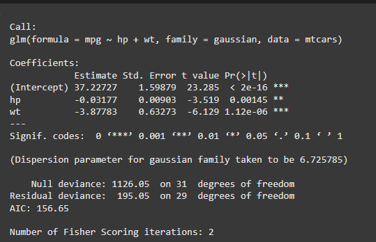
Summary of the model
A one unit hp increase predicts a 0.03177 mpg decrease, while one unit wt increase predicts a 3.87783 mpg decrease.
4. Visualize the model
After creating an extended linear model, we must evaluate its fit to the data. This can be accomplished with the help of diagnostic graphs such as the residual plot and the Q-Q plot.
R `
plot(model, which = 1)
plot(model, which = 2)
`
**Output:

Generalized Linear Models in R
The residual plot displays the residuals (differences between measured and predicted values) plotted against the fitted values. (i.e. the predicted values). We want to see a random scatter of residuals around zero, which indicates that the model is capturing the data trends.

Generalized Linear Models in R
The residuals Q-Q plot displays the residuals plotted against the anticipated values if they were normally distributed. The points should follow a straight line, showing that the residuals are normally distributed.