How to create Kernel Density Plot in R? (original) (raw)

Last Updated : 23 May, 2021

In this article, we will discuss how to create kernel density plots in R programming language. For this, the user simply needs to call the density() function which is an in-build function in R language. Then the user has to pass the given data as the parameter to this function in order to create a density plot of the given data and further in return this function will be returning the density plot of the given data.

By simple variation in the parameter of density() function, the user can enhance the density plot of the given data and a better understandability to it.

Syntax: density(x,…)

Parameters:

• x:-the data from which the estimate is to be computed.
• ...:-further arguments for (non-default) methods.

Returns:

This function will be returning the density plot of the given data.

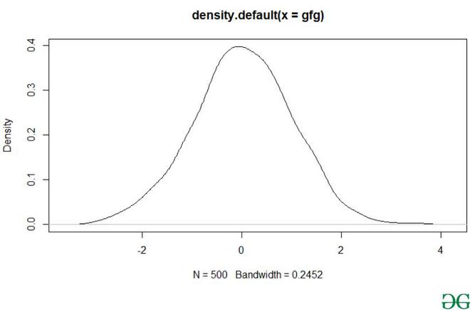
Let us first create a general density plot for some data without any modification for enhancement purposes.

Example:

R `

500 random numeric data

gfg <-rnorm(500)

plot(density(gfg))

`

Output:

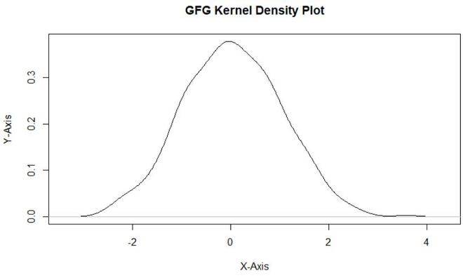
Using the density() function the user can easily plot the kernel density curve in R language, but to modify the main title and the axis label user need to include xlab/ylab as the parameter of the plot function which will help the user to modify the axis label and to modify the main title, the user needs to add main as the parameter of the plot function and this will lead to modification of main title & axis labels of density plot in R language.

• main: an overall title for the plot.
• xlab: a title for the x-axis.
• ylab: a title for the y axis.

Example:

R `

gfg <-rnorm(500)

plot(density(gfg),main = "GFG Kernel Density Plot", xlab = "X-Axis",ylab = "Y-Axis")

`

Output:

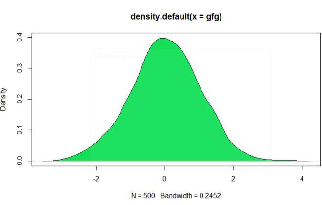
To create a polygon below the density plot, the user needs to use the polygon function in combination with the density function, here the polygon function is used to create the polygon under the density plot and the density() function is used to create the density plot of the given data.

polygon() function helps to draw the polygons whose vertices are given in x and y.

Syntax:

polygon(x, y = NULL, density = NULL, angle = 45,border = NULL, col = NA, lty = par("lty"), …, fillOddEven = FALSE)

Parameters:

• x, y:-vectors containing the coordinates of the vertices of the polygon.
• density:-the density of shading lines, in lines per inch. The default value of NULL means that no shading lines are drawn.
• angle:-the slope of shading lines, given as an angle in degrees (counter-clockwise).
• col:-the color for filling the polygon. The default, NA, is to leave polygons unfilled unless density is specified.
• border:-the color to draw the border. The default, NULL, means to use par("fg"). Use border = NA to omit borders.
• lty:-the line type to be used, as in par.
• …:-graphical parameters such as xpd, lend, ljoin and lmitre can be given as arguments.
• fillOddEven:-logical controlling the polygon shading mode: see below for details. Default FALSE.

Example:

R `

gfg <-rnorm(500)

plot(density(gfg))

polygon(density(gfg), col = "#14e058")

`

Output:

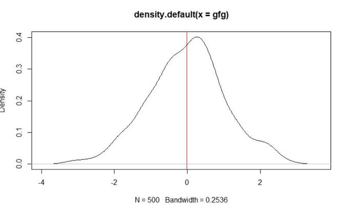
To add a mean line vertically to the density plot user need to call the abline() function with the required parameter with the density function which will be returning a vertical line of the density plot at the mean value of the data.

Syntax:

abline(a = NULL, b = NULL, h = NULL, v = NULL, reg = NULL, coef = NULL, untf = FALSE, ...)

Parameters:

• a, b:-the intercept and slope, single values.
• untf:-logical asking whether to untransform.
• h:-the y-value(s) for horizontal line(s).
• v:-the x-value(s) for vertical line(s).
• coef:-a vector of length two giving the intercept and slope.
• reg:-an object with a coef method. See ‘Details’.
• …:-graphical parameters such as col, lty and lwd

Example:

R `

gfg <-rnorm(500)

plot(density(gfg))

abline(v = mean(gfg), col = "red")

`

Output:

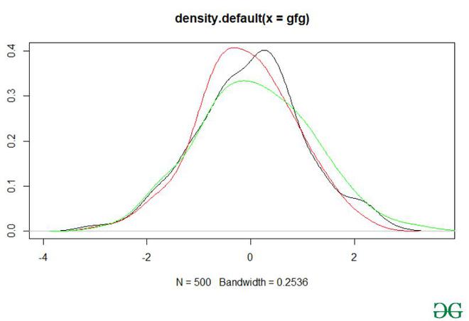
To create multiple kernel density plots in a single plot user need to use the line function with col parameter passed into this function to differentiate among the density plotline and then using the density function to plot the density of all the given multiple plots in a single plot in R language.

lines() is a generic function taking coordinates given in various ways and joining the corresponding points with line segments.

Syntax:

lines(x, …)

Parameters:

• x:-coordinate vectors of points to join.
• …:-Further graphical parameters

Example:

R `

#500 random numeric data gfg <-rnorm(500)

a <- rnorm(200)
b <- rnorm(100)

plot(density(gfg))

lines(density(a), col = "red")
lines(density(b), col = "green")

`

Output:

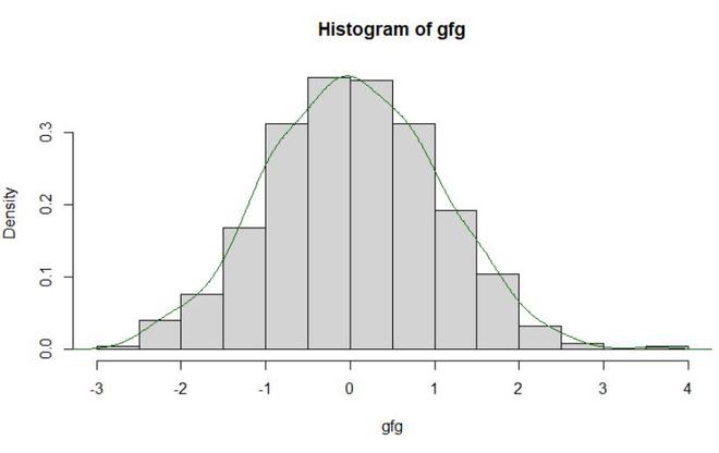
To overlay a histogram with the density plot, the user first needs to call the hist() function with the required parameters pass into it to build the histogram, further, he/she needs to call the density function in the combination of line function to build the density plot of the data in R language.

hist() is a generic function used to compute a histogram of the given data values.

Syntax:

hist(x, …)

Parameters:

• x:-a vector of values for which the histogram is desired.
• …:-further arguments and graphical parameters

Example:

R `

gfg <-rnorm(500)

hist(gfg, prob = TRUE)

lines(density(gfg), col = "#006400")

`

Output: