Hypergeometric Distribution in R Programming (original) (raw)

Last Updated : 15 Jul, 2025

The hypergeometric distribution is a discrete probability distribution that describes the probability of obtaining a certain number of successes in a sequence of draws from a finite population, without replacement. Unlike the binomial distribution, where each draw is independent and with replacement, the hypergeometric distribution considers the fact that each draw affects the subsequent draws.

Key Concepts

• **Finite Population: The hypergeometric distribution applies to situations where you have a finite population consisting of two types of items (successes and failures). The population is divided into two groups:
  • m: The number of successes in the population.
  • n: The number of failures in the population.
• **Sample Without Replacement: A sample of size k is drawn from this population without replacement, meaning that once an item is drawn, it is not returned to the population for subsequent draws.
• **Number of Successes: The random variable of interest, X, represents the number of successes in the sample of size k.

Hypergeometric Functions in R

R provides several functions to work with the hypergeometric distribution:

1. dhyper: Calculates the probability of obtaining exactly x successes in a sample of size k drawn from a population with m successes and n failures.
2. phyper: Computes the cumulative probability of getting q or fewer successes in the sample.
3. qhyper: Finds the quantile corresponding to a given cumulative probability p.
4. rhyper: Generates random samples from a hypergeometric distribution, where nn is the number of samples to generate.

Now we will discuss all the 4 function in detail using R Programming Language.

1. dhyper()

The dhyper() function calculates the probability of getting exactly x successes (items of interest) in a sample of size k, drawn without replacement from a population containing m successes and n failures.

dhyper(x, m, n, k)

Where,

• x: The number of successes in the sample (i.e., the number of items of interest in your sample).
• m: The number of items of interest in the population (i.e., the total number of successes in the population).
• n: The number of items not of interest in the population (i.e., the total number of failures in the population).
• k: The number of items drawn in the sample.

The dhyper() function gives the probability of getting exactly x successes in a sample of size k, drawn from a population with m successes and n failures.

R `

Specify x-values for dhyper function

x_dhyper <- seq(0, 22, by = 1.2)

Apply dhyper function

y_dhyper <- dhyper(x_dhyper, m = 45, n = 30, k = 20)

Plot dhyper values

plot(y_dhyper)

`

**Output:

Hypergeometric Distribution in R Programming

**2: phyper()

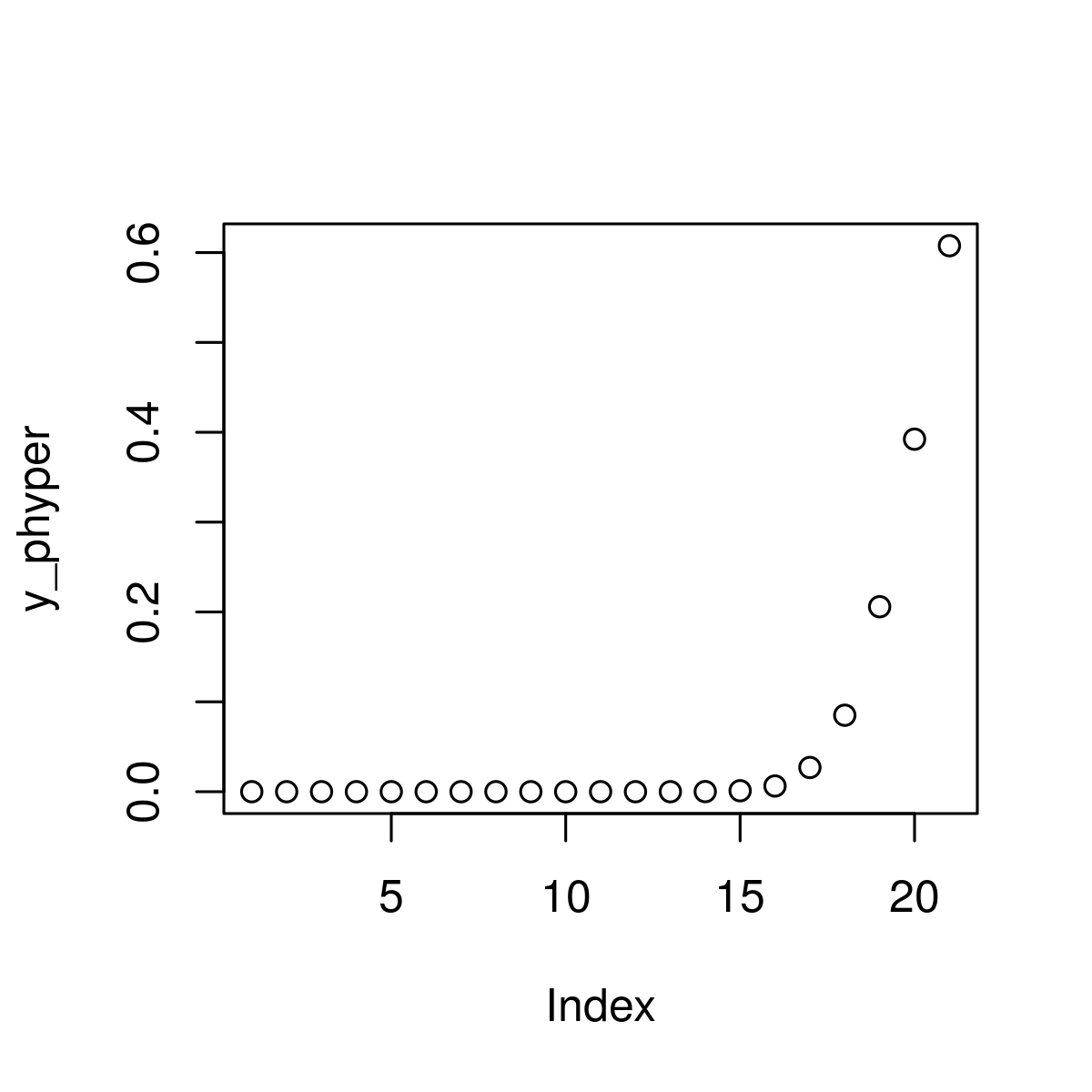
The phyper() function calculates the cumulative probability of getting x or fewer successes in a sample of size k, drawn without replacement from a population containing m successes and n failures. It answers the question, "What is the probability of getting at most x successes?"

phyper(x, m, n, k)

Where,

• x: The number of successes in the sample.
• m: The number of items of interest in the population.
• n: The number of items not of interest in the population.
• k: The number of items drawn in the sample.

The phyper() function calculates the cumulative probability (the probability of getting x or fewer successes) in a hypergeometric distribution.

R `

Specify x-values for phyper function

x_phyper <- seq(0, 22, by = 1)

Apply phyper function

y_phyper <- phyper(x_phyper, m = 40, n = 20, k = 31)

Plot phyper values

plot(y_phyper)

`

**Output:

Hypergeometric Distribution in R Programming

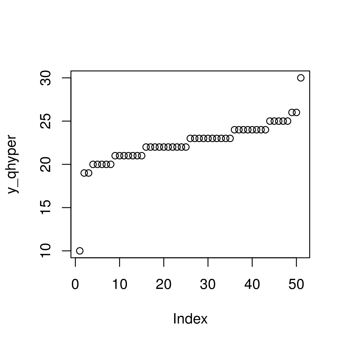
3: **qhyper()

The qhyper() function returns the smallest number x such that the cumulative probability is at least p. In other words, it finds the quantile corresponding to a given cumulative probability.

qhyper(p, m, n, k)

Where,

• p: The cumulative probability.
• m: The number of items of interest in the population.
• n: The number of items not of interest in the population.
• k: The number of items drawn in the sample.

The qhyper() function returns the quantile function (i.e., the smallest number x such that the cumulative probability is at least p).

R `

Specify x-values for qhyper function

x_qhyper <- seq(0, 1, by = 0.02)

Apply qhyper function

y_qhyper <- qhyper(x_qhyper, m = 49, n = 18, k = 30)

Plot qhyper values

plot(y_qhyper)

`

**Output:

Hypergeometric Distribution in R Programming

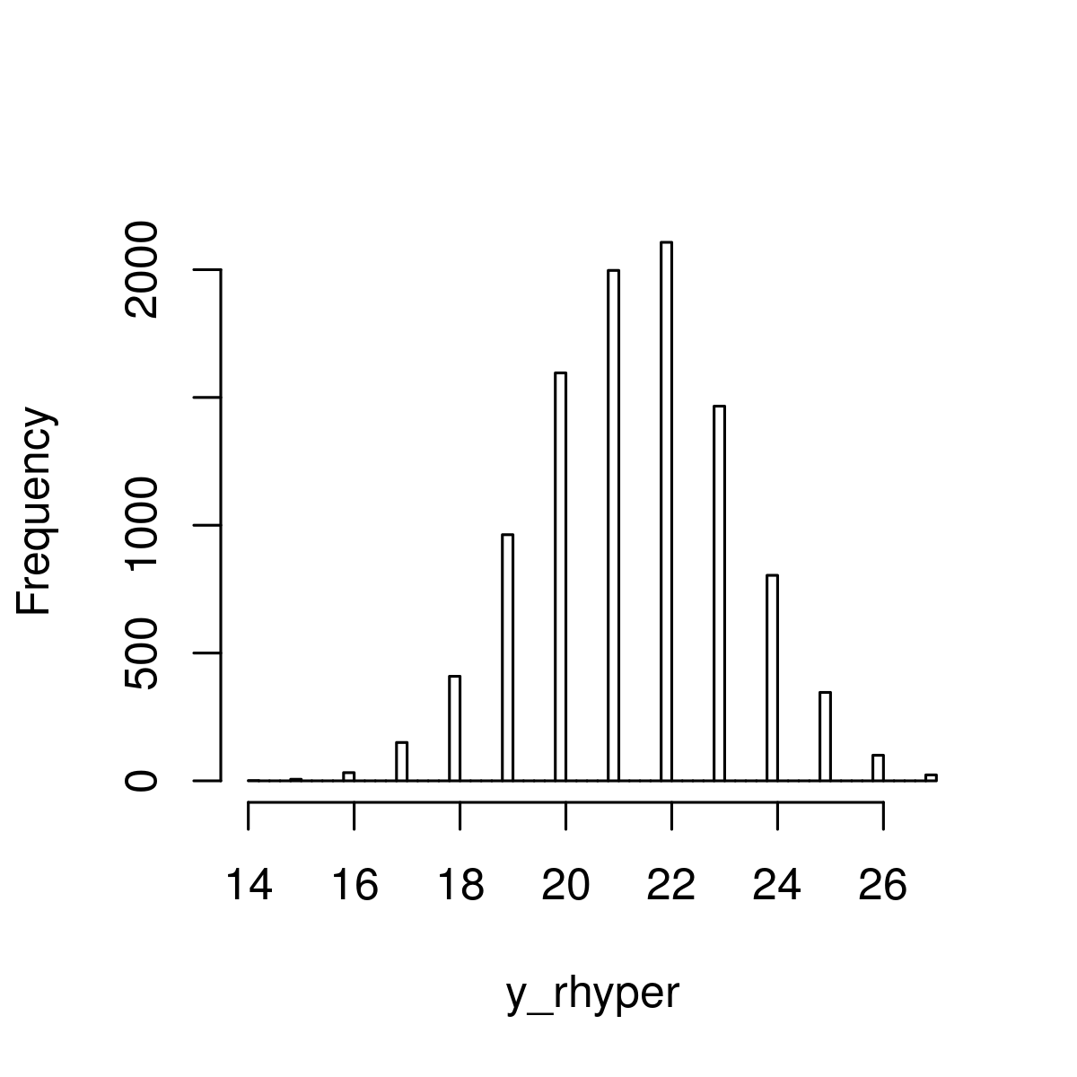
4: **rhyper()

The rhyper() function generates random values from a hypergeometric distribution. It simulates drawing k items from a population containing m successes and n failures, N times.

rhyper(N, m, n, k)

Where,

• N: The number of random values to generate.
• m: The number of items of interest in the population.
• n: The number of items not of interest in the population.
• k: The number of items drawn in each sample.

The rhyper() function generates random values from a hypergeometric distribution.

R `

Set seed for reproducibility

Specify sample size

set.seed(400) N <- 10000

Draw N hypergeometrically distributed values

y_rhyper <- rhyper(N, m = 50, n = 20, k = 30)

Plot of randomly drawn hyper density

hist(y_rhyper, breaks = 50, main = "")

`

**Output:

Hypergeometric Distribution in R Programming

Applications of Hypergeometric Distribution

The hypergeometric distribution is widely used in scenarios where sampling without replacement is relevant. Some common applications include:

• **Quality Control: Determining the probability of finding a certain number of defective items in a batch when sampling without replacement.
• **Ecology: Estimating species diversity by sampling from a finite population of organisms.
• **Card Games: Calculating the probability of drawing a certain hand in games like poker where cards are drawn without replacement.
• **Lottery Games: Modeling the probability of winning by drawing a specific number of matching numbers.

Conclusion

The hypergeometric distribution is a powerful tool in statistical analysis for scenarios involving sampling without replacement from a finite population. Understanding the theory behind the distribution, and how to use R's hypergeometric functions, enables accurate probability calculations in various fields such as quality control, ecology, and gaming.