KNN Classifier in R Programming (original) (raw)

Last Updated : 2 May, 2025

K-Nearest Neighbor or KNN is a supervised non-linear classification algorithm. It is also Non-parametric in nature meaning , it doesn't make any assumption about underlying data or its distribution.

Algorithm Structure

In KNN algorithm, K specifies the number of neighbors and its algorithm is as follows:

• Choose the number K of the neighbor.
• Take the K Nearest Neighbor of unknown data point according to distance.
• Among the K-neighbors, count the number of data points in each category.
• Assign the new data point to a category, where you counted the most neighbors.

For the Nearest Neighbor classifier, the distance between two points is expressed in the form of **Euclidean Distance.

Example:

Consider a dataset containing two features Red and Blue and we classify them. Here K =5 meaning, we are considering 5 neighbors according to Euclidean distance.

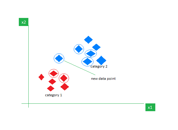
So, when a new data point enters, out of 5 neighbors, if 3 are Blue and 2 are Red, we assign the new data point to the category with most neighbors (in this case that will be Blue).

Implemention of KNN

We will perform the K-Nearest Neighbor Algorithm in R programming language using the Iris dataset.

1. Installing the Required Packages

We will install the **class package which can be used to fit a KNN model also **caTools for splitting our dataset into training and testing.

R `

install.packages("caTools") install.packages("class") install.packages("ggplot2")

library(caTools) library(class) library(ggplot2)

`

2. Importing the Dataset

We will use the Iris dataset which is a built in dataset in R programming language which contains 50 samples from each of 3 species of Iris(Iris setosa, Iris virginica, Iris versicolor). We will use the str() function to give us the feature names and structure of the dataset.

R `

data(iris) str(iris)

`

**Output:

Structure of the data

3. Splitting data into train and test data

We first split the iris dataset into training and testing sets using a 70:30 ratio. Then, we scale the numeric feature columns (first 4) in both sets to normalize their values.

R `

split <- sample.split(iris, SplitRatio = 0.7) train_cl <- subset(iris, split == "TRUE") test_cl <- subset(iris, split == "FALSE")

train_scale <- scale(train_cl[, 1:4]) test_scale <- scale(test_cl[, 1:4])

`

4. Fitting KNN Model

We fit a KNN model using the scaled training data, where**k = 1**. The model then predicts species labels for the test set based on the nearest neighbor from the training set. Also, the Classifier Species feature is fitted in the model.

R `

classifier_knn <- knn(train = train_scale, test = test_scale, cl = train_cl$Species, k = 1)

`

5. Displaying a Confusion Matrix

We create a confusion matrix to compare the predicted labels with the actual species in the test set. This helps us evaluate how well the KNN model classified each species.

R `

cm <- table(test_cl$Species, classifier_knn) cm

`

**Output:

Confusion Matrix of the KNN model

6. Evaluating the Model for different K values

We test multiple values of **k to find the most suitable one for our KNN model. For each k, we calculate the miss-classification error and print the corresponding accuracy. This helps in selecting a k that balances bias and variance for better model performance.

R `

library(ggplot2)

k_values <- c(1, 3, 5, 7, 15, 19)

accuracy_values <- sapply(k_values, function(k) { classifier_knn <- knn(train = train_scale, test = test_scale, cl = train_cl$Species, k = k) 1 - mean(classifier_knn != test_cl$Species) })

accuracy_data <- data.frame(K = k_values, Accuracy = accuracy_values)

ggplot(accuracy_data, aes(x = K, y = Accuracy)) + geom_line(color = "lightblue", size = 1) + geom_point(color = "lightgreen", size = 3) + labs(title = "Model Accuracy for Different K Values", x = "Number of Neighbors (K)", y = "Accuracy") + theme_minimal()

`

**Output:

KNN model performance

From the graph, we observe the following accuracy trends for different values of **k:

• **k = 1: The model achieved **91.66% accuracy.
• **k = 3: The accuracy remained the same at **91.66%, showing no improvement over k = 1.
• **k = 5: Accuracy increased to **95%, which is higher than at k = 1 and 3.
• **k = 7: The accuracy remained **95%, same as at k = 5.
• **k = 15: The accuracy dropped slightly to **92.5%.
• **k = 19: The accuracy further decreased to **90%, the lowest among all tested values.

Therefore, the optimal value of k for our model is 5.

In this article, we implemented the K-Nearest Neighbors (KNN) algorithm on the iris dataset and evaluated model accuracy across different values of k. We found that accuracy peaked at k = 5 and 7, demonstrating the importance of tuning k for optimal performance.