Linear Discriminant Analysis in R Programming (original) (raw)

Last Updated : 14 Apr, 2026

Linear Discriminant Analysis (LDA) is a statistical method that is also widely used in machine learning for classification and dimensionality reduction. It works by finding a line (or plane in higher dimensions) that best separates the classes in the data by creating linear combinations of input features to maximize the distance between classes and minimize variation within the same class.

Assumptions of Linear Discriminant Analysis (LDA)

The features are normally distributed (Gaussian).
All classes share equal covariance.
The target (dependent) variable is categorical.

Where is LDA Used?

LDA is widely applied in various real-world scenarios, including:

**Face Recognition: Used to reduce the dimensionality of facial images before performing classification.
**Customer Behavior Analysis: Helps identify key features that influence purchasing decisions.
**Medical Diagnosis: Assists in classifying patient cases into categories such as mild, moderate or severe.
**Marketing and Segmentation: Used to group customers based on their preferences or spending habits.

Implementation of Linear Discriminant Analysis (LDA)

We implement Linear Discriminant Analysis using the lda() function from the MASS package on the Iris dataset and visualize class separation with synthetic data.

1. Installing and Loading Required Packages

We install and load all required packages to preprocess data, build the model and visualize results.

**install.packages: used to install external packages.
**library: loads the installed package into the R session.
**MASS: Statistical models, linear/discriminant analysis, example datasets.
**tidyverse: Collection of data science packages (dplyr, ggplot2, readr, etc.).
**caret: Machine learning framework for training, tuning, validation.
**mvtnorm: Functions for multivariate normal and t-distributions.
**ggplot2: Grammar-based plotting system for data visualization. R `

install.packages("MASS") install.packages("tidyverse") install.packages("caret") install.packages("mvtnorm")

library(MASS) library(tidyverse) library(caret) library(mvtnorm) library(ggplot2)

2. Loading and Splitting the Dataset

We load the Iris dataset and divide it into training and test sets.

**data: Loads a built-in dataset (e.g., iris).
**createDataPartition: Splits the dataset into training and test sets with balanced class distribution.
**set.seed: Sets a seed value to ensure reproducible results across runs. R `

data("iris") set.seed(123) training.individuals <- iris$Species %>% createDataPartition(p = 0.8, list = FALSE) train.data <- iris[training.individuals, ] test.data <- iris[-training.individuals, ]

3. Normalizing the Dataset

Normalization is not strictly required for LDA, but it can help when features are on very different scales.

**preProcess: estimates the normalization parameters.
**predict: applies those parameters to transform the dataset. R `

preproc.parameter <- train.data %>% preProcess(method = c("center", "scale")) train.transform <- preproc.parameter %>% predict(train.data) test.transform <- preproc.parameter %>% predict(test.data)

4. Fitting the LDA Model

We train the LDA model using the transformed training dataset.

**lda(): fits the Linear Discriminant Analysis model.
**Species ~ .: means all variables are used to predict species. R `

model <- lda(Species ~ ., data = train.transform)

5. Making Predictions

We use the model to predict species on the test set.

**predict(): generates class predictions and related values. R `

predictions <- model %>% predict(test.transform)

6. Checking Model Accuracy

We calculate how many predictions matched the actual labels.

**mean(): computes the accuracy by checking prediction correctness. R `

mean(predictions$class == test.transform$Species)

**Output:

0.966666666666667

7. Viewing Model Details

We print the model output including prior probabilities, group means and coefficients.

**model: shows the internal summary of the LDA model. R `

model

**Output:

dataset

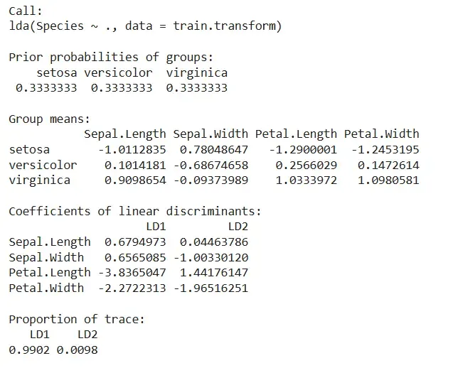
Output

8. Plotting the Output

We generate synthetic Gaussian samples to visualize how well LDA can separate two classes.

**matrix(): defines the covariance between features.
**rmvnorm(): creates random multivariate normal samples.
**cbind / rbind: combines datasets.
**geom_point(): adds data points to the plot colored by class. R `

var_covar <- matrix(data = c(1.5, 0.4, 0.4, 1.5), nrow = 2) Xplus1 <- rmvnorm(400, mean = c(5, 5), sigma = var_covar) Xminus1 <- rmvnorm(600, mean = c(3, 3), sigma = var_covar) Y_samples <- c(rep(1, 400), rep(-1, 600)) dataset <- as.data.frame(cbind(rbind(Xplus1, Xminus1), Y_samples)) colnames(dataset) <- c("X1", "X2", "Y") dataset$Y <- as.character(dataset$Y)

ggplot(data = dataset) + geom_point(aes(X1, X2, color = Y))

**Output:

graph-output

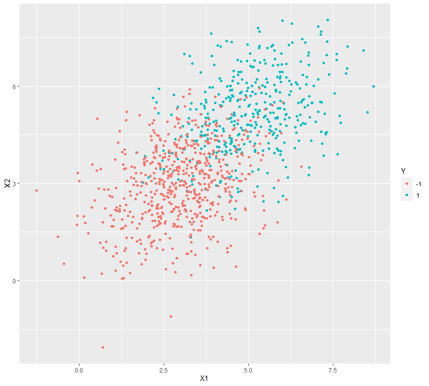
The output is a scatter plot showing two distinct classes of synthetic data points, where each class forms a cluster, helping visualize how LDA can separate them based on feature values.