Linear Regression in R (original) (raw)

Last Updated : 1 Jul, 2025

Linear regression is a statistical approach used to model the relationship between a dependent variable and one or more independent variables. A straight line is assumed to approximate this relationship. The goal is to identify the line that minimizes discrepancies between the observed data points and predicted values.

There are two main types of linear regression:

• **Simple Linear Regression (single dependent variable, single independent variable)
• **Multiple Linear Regression (single dependent variable, multiple independent variables)

Linear Regression Line

A regression line shows the relationship between the dependent and independent variables. It can either exhibit:

• **Positive Linear Relationship: As the independent variable increases, the dependent variable increases.
• **Negative Linear Relationship: As the independent variable increases, the dependent variable decreases.

Assumptions of Linear Regression

Linear regression algorithm assumes the following:

1. **Linear relationship: The dependent and independent variables are linearly related.
2. **No multicollinearity: Independent variables should not be highly correlated.
3. **Homoscedasticity: The error term should remain constant across all levels of the independent variables.
4. **Normal distribution of error terms: Error terms should follow a normal distribution.
5. **No autocorrelation: The error terms should not show patterns.

Mathematically

The linear regression equation is:

Y = \beta_0 + \beta_1X + \epsilon

**Where:

• Y is the dependent variable.
• X is the independent variable.
• \beta_0 is the intercept.
• \beta_1 is the slope of the line.
• \epsilon is the error term.

Implementation of Linear Regression in R

In this section, we will load the dataset, split it into training and test sets and build a linear regression model to predict salaries based on years of experience.

1. Installing Required Libraries

We will install and load the caTools library for dataset splitting and ggplot2 for visualizations.

• **install.packages(): Installs the libraries.
• **library(): Loads the libraries to be used. R `

install.packages('caTools') install.packages("ggplot2")

library(ggplot2) library(caTools)

`

2. Loading the Dataset

We will create a sample dataset (salary dataset ) and load it into R as a data frame. We will also display it

• **data.frame(): Converts the given vectors of years and salaries into a data frame.
• **plot(): Plots a graph to visualize our data. R `

data <- data.frame( YearsExperience = c(1.1, 1.3, 1.5, 10.3, 10.5, 2.0, 2.2, 2.9, 3.0, 3.2, 3.2, 3.7, 3.9, 4.0, 4.0, 4.1, 4.5, 4.9, 5.1, 5.3, 5.9, 6.0, 6.8, 7.1, 7.9, 8.2, 8.7, 9.0, 9.5, 9.6), Salary = c(39343.00, 46205.00, 37731.00, 122391.00, 121872.00, 43525.00, 39891.00, 56642.00, 60150.00, 54445.00, 64445.00, 57189.00, 63218.00, 55794.00, 56957.00, 57081.00, 61111.00, 67938.00, 66029.00, 83088.00, 81363.00, 93940.00, 91738.00, 98273.00, 101302.00, 113812.00, 109431.00, 105582.00, 116969.00, 112635.00) )

plot(data)

`

**Output:

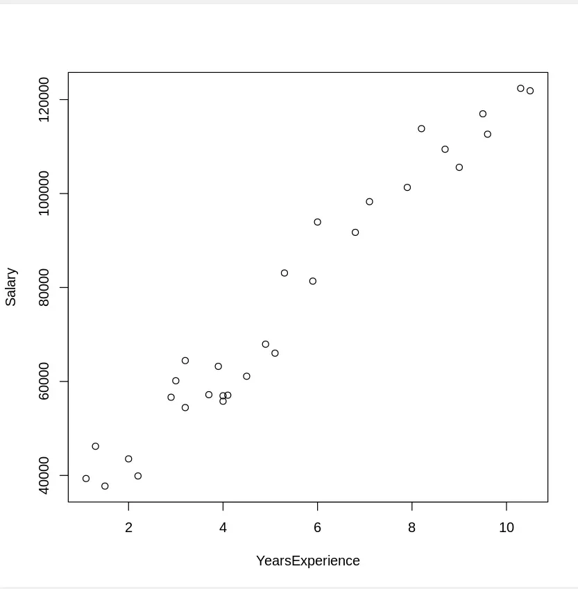
Dataset

3. Splitting the Dataset

We will split the dataset into training and test sets.

• **sample.split(): Splits the dataset into training and test sets based on a given split ratio (70% for training).
• **subset(): Selects the appropriate data for the training and test sets. R `

split = sample.split(data$Salary, SplitRatio = 0.7) trainingset = subset(data, split == TRUE) testset = subset(data, split == FALSE)

`

4. Building the Linear Regression Model

We will now build the simple linear regression model using the training set.

• **lm(): Fits a linear model, where Salary ~ YearsExperience represents the formula to predict salary based on years of experience. The formula represents the regression model (dependent ~ independent). R `

lm_r = lm(formula = Salary ~ Years_Exp, data = trainingset)

`

5. Model Summary

After fitting the model, we will view the summary to understand the coefficients and statistical significance.

• **summary(): Displays the summary of the linear model, including coefficients, residuals and goodness-of-fit statistics. R `

summary(lm_r)

`

**Output:

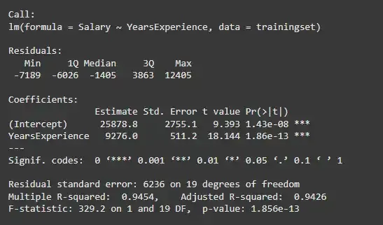
Model Summary

6. Visualization of Results

We will visualize the model's performance by plotting the training and test sets.

• **geom_point(): Creates the scatter plot for the dataset.
• **geom_line(): Plots the regression line over the data points.
• **ggtitle(), xlab(), ylab(): Adds titles and labels to the plot.

6.1. Training Set Visualization:

R `

ggplot() + geom_point(aes(x = trainingset$YearsExperience, y = trainingset$Salary), colour = 'red') + geom_line(aes(x = trainingset$YearsExperience, y = predict(lm_r, newdata = trainingset)), colour = 'blue') + ggtitle('Salary vs Experience (Training set)') + xlab('Years of experience') + ylab('Salary')

`

Output:

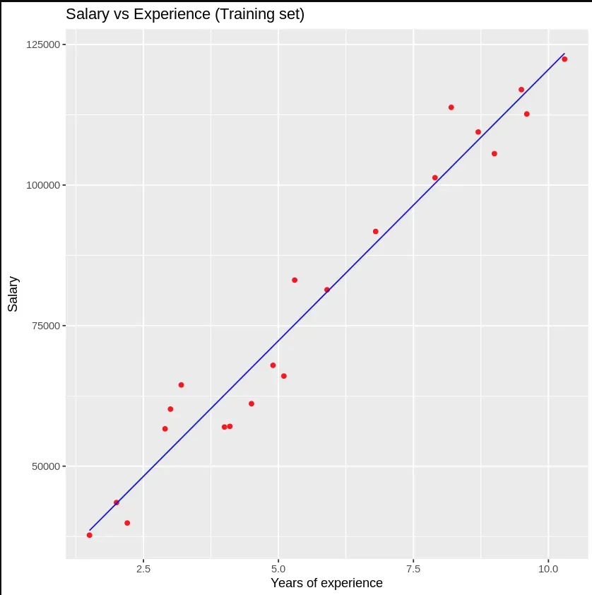
Training Set Visualization:

6.2. Test Set Visualization:

R `

ggplot() + geom_point(aes(x = testset$YearsExperience, y = testset$Salary), colour = 'red') + geom_line(aes(x = trainingset$YearsExperience, y = predict(lm_r, newdata = trainingset)), colour = 'blue') + ggtitle('Salary vs Experience (Test set)') + xlab('Years of experience') + ylab('Salary')

`

Output:

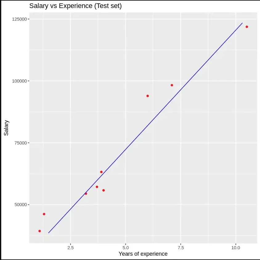
Test Set Visualization

7. Making Predictions

We will predict salary values based on new input years of experience.

• **predict(): Uses the trained model to make predictions for new data. R `

new_data <- data.frame(YearsExperience = c(4.0, 4.5, 5.0)) predicted_salaries <- predict(lm_r, newdata = new_data) print(predicted_salaries)

`

**Output:

1 2 3

62983.00 67621.02 72259.04

Advantages of Linear Regression in R:

• **Easy to Implement: Built-in functions like **lm() make it straightforward.
• **Interpretable: Simple Linear Regression provides easy-to-understand results.
• **Useful for Prediction: It can predict numeric variables like salary, price, etc.

Disadvantages:

• **Assumes a Linear Relationship: The assumption of linearity may not hold true in all cases.
• **Sensitive to Outliers: Outliers can significantly affect the model's accuracy.
• **Requires Numeric Data: It cannot handle categorical or non-numeric data.

In this article, we implemented Linear Regression in R to predict salary based on years of experience. The model fit the data well and predictions for new data were successfully made. We also visualized the model’s performance using plots.